
Highlights §
- Because these huge models require so many GPUs to run, we need to find ways to reduce these requirements while preserving the model’s performance. Various technologies have been developed that try to shrink the model size, you may have heard of quantization and distillation, and there are many others. (View Highlight)
- After completing the training of BLOOM-176B, we at HuggingFace and BigScience were looking for ways to make this big model easier to run on less GPUs. Through our BigScience community we were made aware of research on Int8 inference that does not degrade predictive performance of large models and reduces the memory footprint of large models by a factor or 2x. Soon we started collaboring on this research which ended with a full integration into Hugging Face
transformers. With this blog post, we offer LLM.int8() integration for all Hugging Face models which we explain in more detail below. (View Highlight)
- We start with the basic understanding of different floating point data types, which are also referred to as “precision” in the context of Machine Learning. (View Highlight)
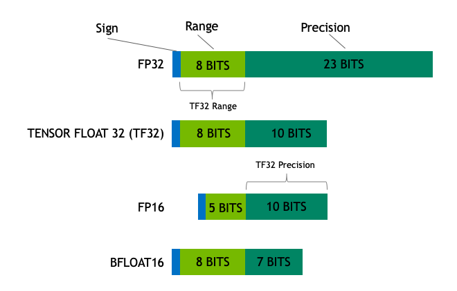
- The size of a model is determined by the number of its parameters, and their precision, typically one of float32, float16 or bfloat16 (image below from: https://blogs.nvidia.com/blog/2020/05/14/tensorfloat-32-precision-format/).
 (View Highlight)
- Float32 (FP32) stands for the standardized IEEE 32-bit floating point representation. With this data type it is possible to represent a wide range of floating numbers. In FP32, 8 bits are reserved for the “exponent”, 23 bits for the “mantissa” and 1 bit for the sign of the number. In addition to that, most of the hardware supports FP32 operations and instructions. (View Highlight)
- In the float16 (FP16) data type, 5 bits are reserved for the exponent and 10 bits are reserved for the mantissa. This makes the representable range of FP16 numbers much lower than FP32. This exposes FP16 numbers to the risk of overflowing (trying to represent a number that is very large) and underflowing (representing a number that is very small).
For example, if you do
10k * 10k you end up with 100M which is not possible to represent in FP16, as the largest number possible is 64k. And thus you’d end up with NaN (Not a Number) result and if you have sequential computation like in neural networks, all the prior work is destroyed. Usually, loss scaling is used to overcome this issue, but it doesn’t always work well.
A new format, bfloat16 (BF16), was created to avoid these constraints. In BF16, 8 bits are reserved for the exponent (which is the same as in FP32) and 7 bits are reserved for the fraction.
This means that in BF16 we can retain the same dynamic range as FP32. But we lose 3 bits of precision with respect to FP16. Now there is absolutely no problem with huge numbers, but the precision is worse than FP16 here. (View Highlight)
- In the Ampere architecture, NVIDIA also introduced TensorFloat-32 (TF32) precision format, combining the dynamic range of BF16 and precision of FP16 to only use 19 bits. It’s currently only used internally during certain operations.
In the machine learning jargon FP32 is called full precision (4 bytes), while BF16 and FP16 are referred to as half-precision (2 bytes). On top of that, the int8 (INT8) data type consists of an 8-bit representation that can store 2^8 different values (between [0, 255] or [-128, 127] for signed integers). (View Highlight)
- While, ideally the training and inference should be done in FP32, it is two times slower than FP16/BF16 and therefore a mixed precision approach is used where the weights are held in FP32 as a precise “main weights” reference, while computation in a forward and backward pass are done for FP16/BF16 to enhance training speed. The FP16/BF16 gradients are then used to update the FP32 main weights.
During training, the main weights are always stored in FP32, but in practice, the half-precision weights often provide similar quality during inference as their FP32 counterpart — a precise reference of the model is only needed when it receives multiple gradient updates. This means we can use the half-precision weights and use half the GPUs to accomplish the same outcome. (View Highlight)
- To calculate the model size in bytes, one multiplies the number of parameters by the size of the chosen precision in bytes. For example, if we use the bfloat16 version of the BLOOM-176B model, we have
176*10**9 x 2 bytes = 352GB! (View Highlight)
- Experimentially, we have discovered that instead of using the 4-byte FP32 precision, we can get an almost identical inference outcome with 2-byte BF16/FP16 half-precision, which halves the model size. It’d be amazing to cut it further, but the inference quality outcome starts to drop dramatically at lower precision.
To remediate that, we introduce 8-bit quantization. This method uses a quarter precision, thus needing only 1/4th of the model size! But it’s not done by just dropping another half of the bits. (View Highlight)
- Quantization is done by essentially “rounding” from one data type to another. For example, if one data type has the range 0..9 and another 0..4, then the value “4” in the first data type would be rounded to “2” in the second data type. However, if we have the value “3” in the first data type, it lies between 1 and 2 of the second data type, then we would usually round to “2”. This shows that both values “4” and “3” of the first data type have the same value “2” in the second data type. This highlights that quantization is a noisy process that can lead to information loss, a sort of lossy compression. (View Highlight)
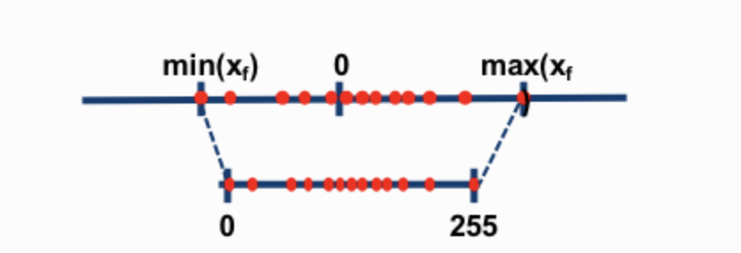
- The two most common 8-bit quantization techniques are zero-point quantization and absolute maximum (absmax) quantization. Zero-point quantization and absmax quantization map the floating point values into more compact int8 (1 byte) values. First, these methods normalize the input by scaling it by a quantization constant. (View Highlight)
- For example, in zero-point quantization, if my range is -1.0…1.0 and I want to quantize into the range -127…127, I want to scale by the factor of 127 and then round it into the 8-bit precision. To retrieve the original value, you would need to divide the int8 value by that same quantization factor of 127. For example, the value 0.3 would be scaled to
0.3*127 = 38.1. Through rounding, we get the value of 38. If we reverse this, we get 38/127=0.2992 – we have a quantization error of 0.008 in this example. These seemingly tiny errors tend to accumulate and grow as they get propagated through the model’s layers and result in performance degradation.
 (View Highlight)
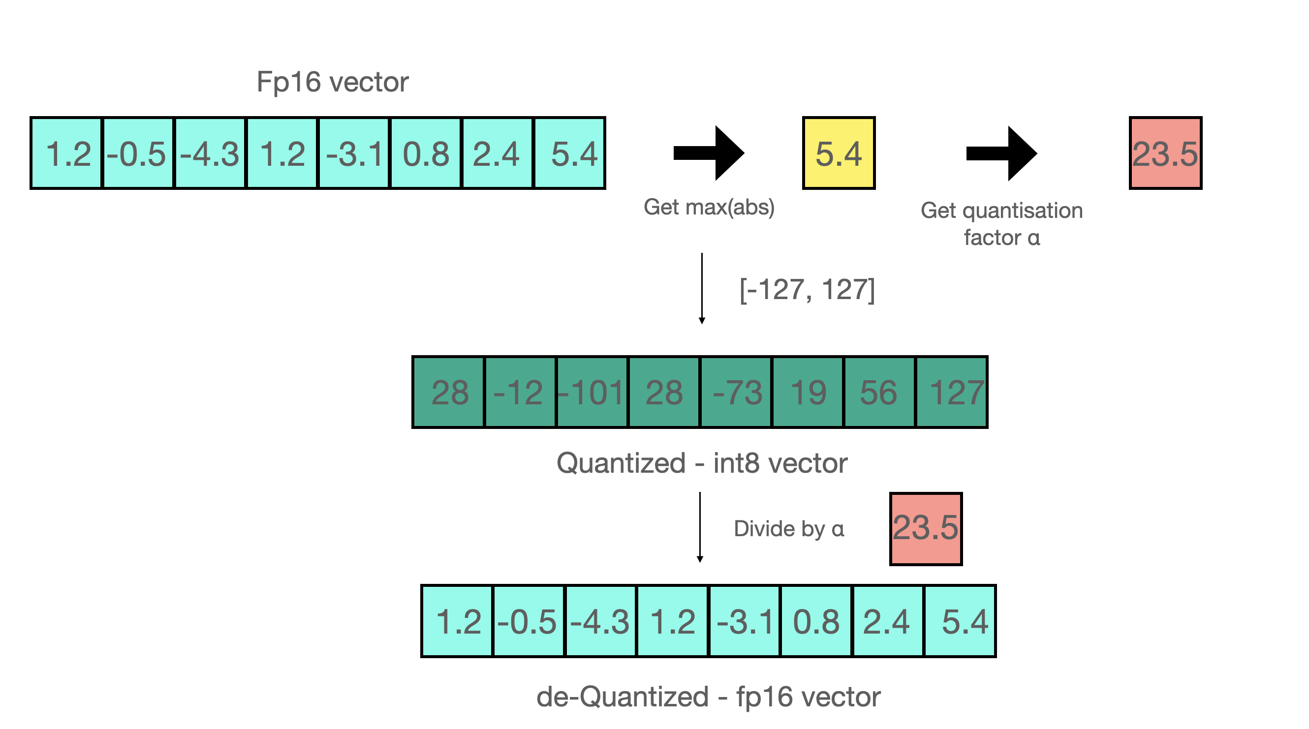
- For example, let’s assume you want to apply absmax quantization in a vector that contains
[1.2, -0.5, -4.3, 1.2, -3.1, 0.8, 2.4, 5.4]. You extract the absolute maximum of it, which is 5.4 in this case. Int8 has a range of [-127, 127], so we divide 127 by 5.4 and obtain 23.5 for the scaling factor. Therefore multiplying the original vector by it gives the quantized vector [28, -12, -101, 28, -73, 19, 56, 127].
 To retrieve the latest, one can just divide in full precision the int8 number with the quantization factor, but since the result above is “rounded” some precision will be lost.
 (View Highlight)
- For an unsigned int8, we would subtract the minimum and scale by the absolute maximum. This is close to what zero-point quantization does. It’s is similar to a min-max scaling but the latter maintains the value scales in such a way that the value “0” is always represented by an integer without any quantization error.
These tricks can be combined in several ways, for example, row-wise or vector-wise quantization, when it comes to matrix multiplication for more accurate results. Looking at the matrix multiplication, AB=C, instead of regular quantization that normalize by a absolute maximum value per tensor, vector-wise quantization finds the absolute maximum of each row of A and each column of B. Then we normalize A and B by dividing these vectors. We then multiply AB to get C. Finally, to get back the FP16 values, we denormalize by computing the outer product of the absolute maximum vector of A and B. (View Highlight)
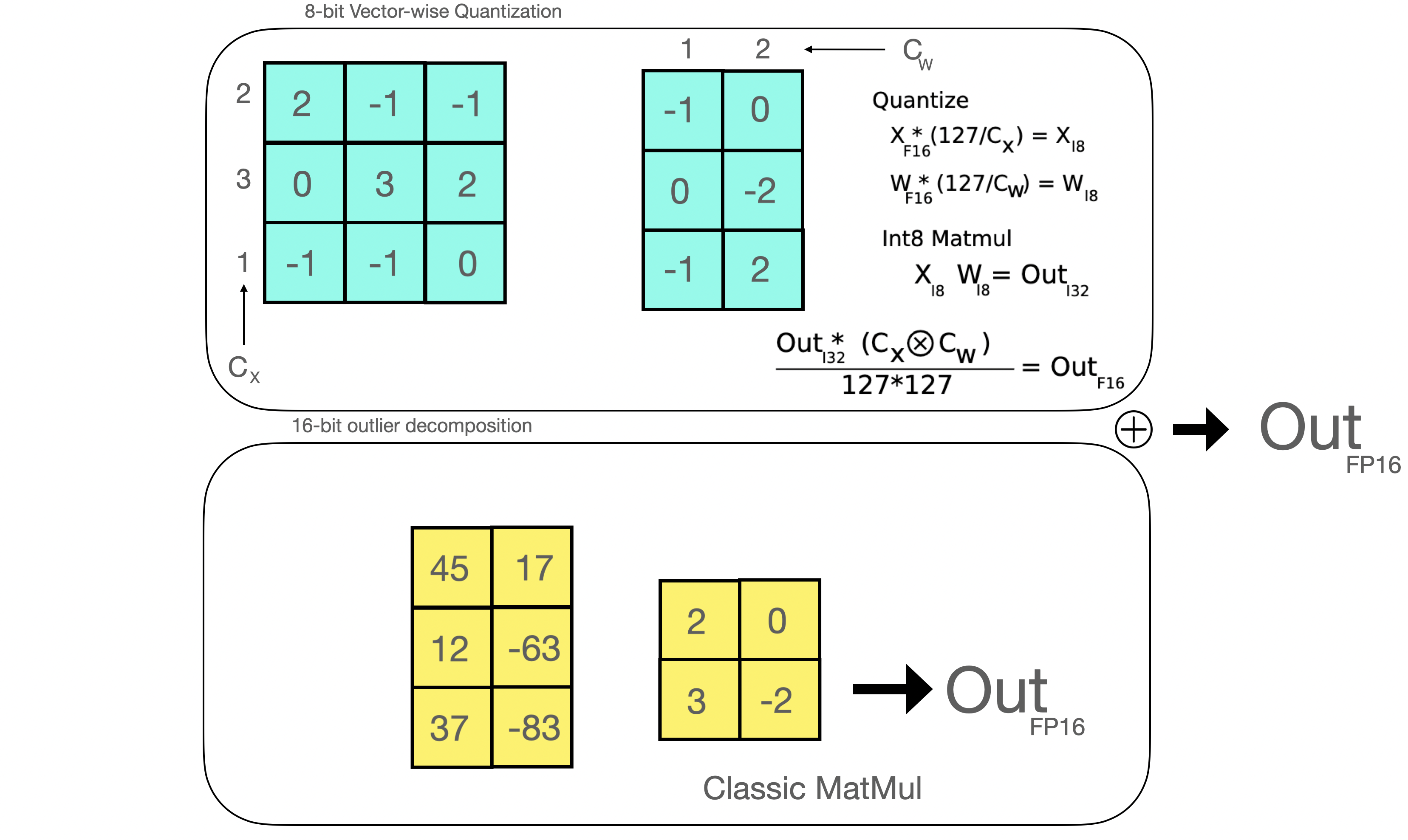
- In LLM.int8(), we have demonstrated that it is crucial to comprehend the scale-dependent emergent properties of transformers in order to understand why traditional quantization fails for large models. We demonstrate that performance deterioration is caused by outlier features, which we explain in the next section. The LLM.int8() algorithm itself can be explain as follows.
In essence, LLM.int8() seeks to complete the matrix multiplication computation in three steps:
- From the input hidden states, extract the outliers (i.e. values that are larger than a certain threshold) by column.
- Perform the matrix multiplication of the outliers in FP16 and the non-outliers in int8.
- Dequantize the non-outlier results and add both outlier and non-outlier results together to receive the full result in FP16.
These steps can be summarized in the following animation:
 (View Highlight)
- A value that is outside the range of some numbers’ global distribution is generally referred to as an outlier. Outlier detection has been widely used and covered in the current literature, and having prior knowledge of the distribution of your features helps with the task of outlier detection. More specifically, we have observed that classic quantization at scale fails for transformer-based models >6B parameters. While large outlier features are also present in smaller models, we observe that a certain threshold these outliers from highly systematic patterns across transformers which are present in every layer of the transformer. (View Highlight)
- Once the hidden states are computed we extract the outliers using a custom threshold and we decompose the matrix into two parts as explained above. We found that extracting all outliers with magnitude 6 or greater in this way recoveres full inference performance. The outlier part is done in fp16 so it is a classic matrix multiplication, whereas the 8-bit matrix multiplication is done by quantizing the weights and hidden states into 8-bit precision using vector-wise quantization — that is, row-wise quantization for the hidden state and column-wise quantization for the weight matrix. After this step, the results are dequantized and returned in half-precision in order to add them to the first matrix multiplication.
 (View Highlight)