Highlights §
- Of all possible activation functions, most people struggle to intuitively understand how ReLU adds non-linearity to a neural network. (View Highlight)
- The confusion is quite obvious because, with its seemingly linear shape, calling it a non-linear activation function isn’t that intuitive. (View Highlight)
- “How does ReLU allow a neural network to capture non-linearity?”
If you have ever struggled with this, then today, let me provide an intuitive explanation as to why ReLU is considered a non-linear activation function. (View Highlight)
- Effectively, it’s the same ReLU function but shifted
h units to the right:
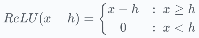 Keep this in mind as we’ll return to it shortly.
Breaking down the output of a neural network (View Highlight)
Keep this in mind as we’ll return to it shortly.
Breaking down the output of a neural network (View Highlight)
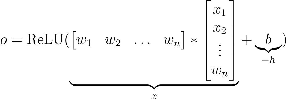
- • First, we have input from the previous layer (x₁, x₂, …, xₙ).
• This is multiplied element-wise by the weights (w₁, w₂, …, wₙ).
• Next, the bias term (
b) is added, and every neuron has its own bias term.
• The above output is passed through an activation function (ReLU in this case) to get the output activation of a neuron. (View Highlight)
- If we notice closely, this final output activation of a neuron is analogous to the
ReLU(x−h) function we discussed earlier.
(View Highlight)
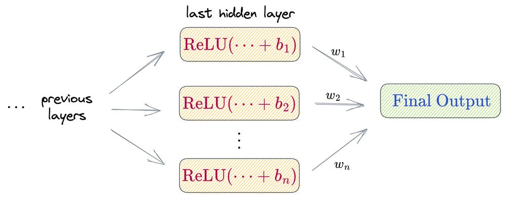
 Now, let’s zoom out and consider all neurons in the last hidden layer. (View Highlight)
- The following image illustrates how neurons in this layer collectively contribute to the network’s output.
 (View Highlight)
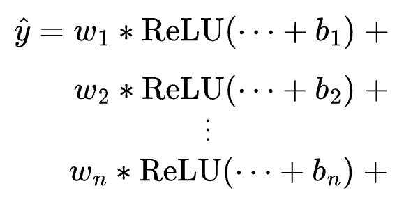
- Essentially, the final output is a weighted sum of differently shifted ReLU activations computed in the last hidden layer.
 (View Highlight)
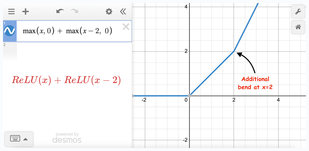
- Now that we know what makes up the final output of a network, let’s plot the weighted sum of some dummy differently shited ReLU functions and see how the plot looks.
Let’s start with two terms:
 (View Highlight)
- In the above image, we notice that adding two ReLU terms changes the slope at a point.
Let’s add more ReLU terms to this.
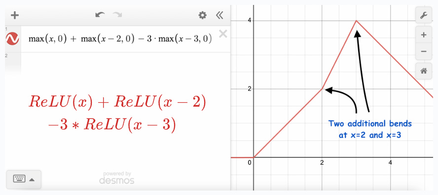 This time, we see two bends in the final output function. (View Highlight)
- The above illustrations depict that we can potentially add more and more ReLU terms, each shifted and multiplied by some constant to get any shape of the curve, linear or non-linear.
 (View Highlight)
- The above equation has no restriction on the nature of the curve; it may be linear or non-linear.
The task is to find those specific weights (w₁, w₂, …, wₙ) which closely estimate the function
f(x).
Theoretically, the precision of approximation can be entirely perfect if we add a ReLU term for each possible value of x. (View Highlight)
- The core point to understand here is that ReLU NEVER adds perfect non-linearity to a neural network.
Instead, it’s the piecewise linearity of ReLU that gives us a perception of a non-linear curve.
Also, as we saw above, the strength of ReLU lies not in itself but in an entire army of ReLUs embedded in the network.
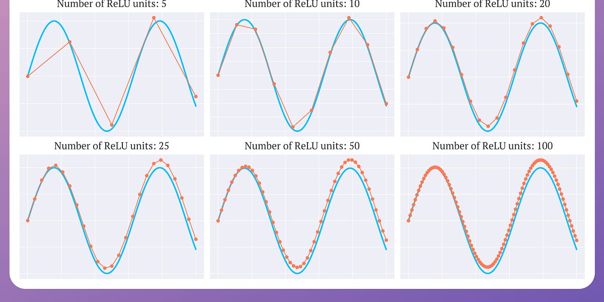
This is why having a few ReLU units in a network may not yield satisfactory results. (View Highlight)
- As shown above, as the number of ReLU units increases, the approximation also becomes better. At 100 ReLU units, the approximation appears entirely non-linear.
And this is precisely why ReLU is called a non-linear activation function. (View Highlight)