
Highlights §
- With just a handful of examples, a fine-tuned open source embedding model can provide greater accuracy at a lower price than proprietary models like OpenAI’s
text-embedding-3-small. In this article, we’ll explain how to create one with Modal. First, we’ll cover the basics of fine-tuning. Then, we’ll talk about an experiment we ran to determine how much fine-tuning data we needed for a simple question-answering use case. (View Highlight)
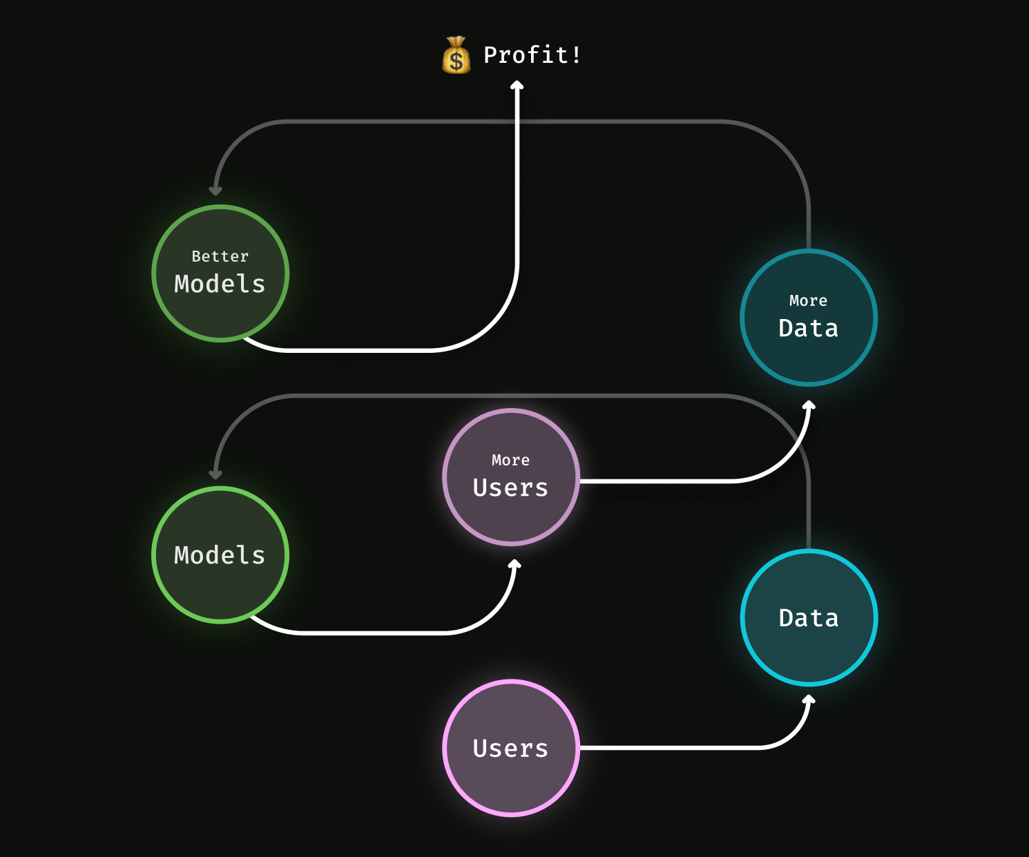
- Custom models matter. That’s how Netflix keeps suggesting better movies and how Spotify manages to find a new anthem for your daylist. By tracking when you finish the movie you chose or whether you skipped a song, these companies accumulate data. They use that data to improve their internal embedding models and recommendation systems, which lead to better suggestions and a better experience for you. That can even lead to more engagement from more users, leading to more data, leading to better models, in a virtuous cycle known as the data flywheel. (View Highlight)
 (View Highlight)
- (View Highlight)
- The data flywheel: more users means more data means better models means more users. (View Highlight)
- The same scalable, serverless infrastructure on Modal that we used to create embeddings with the off-the-shelf model can also be used to customize it, a process called fine-tuning. The end result is an ML application with superior performance at a significantly reduced operational expense: the first step to starting your own data flywheel. (View Highlight)
- Though much of the discussion and research in machine learning is around models, any ML engineer worth their salt will tell you that the dataset is the most critical component. (View Highlight)
- Embedding models are generally trained on datasets made out of pairs of items, where some pairs are marked as “similar” (like sentences from the same paragraph) and some are marked as “different” (like two sentences chosen at random). The same principle could be applied to longer texts than sentences — paragraphs, pages, documents — or it could be applied to things other than text — images, songs, user clickstreams — or it could be applied to multiple modalities at once — images and their captions, songs and their lyrics, user clickstreams and purchased products. (View Highlight)
- You can review the dataset in an interactive viewer here. Some of the question pairs, like “Can I hack my Charter Motorolla DCX3400?” and “How do I hack Motorola DCX3400 for free internet?”, are quite similar, but are not duplicates, aka they are “hard negatives”. (View Highlight)
- Together, that makes the model we’re training here potentially useful for retrieval-augmented generation (RAG) chatbots. In embedding-based RAG for chatbots, a large corpus of text must be searched for a small number of passages that “match” a query from a user, aka likely contain the answer. This dataset will train the model to be sensitive to very small differences in the topic of a question. Near duplicates can also be removed before retrieval or before training other models, a technique known as “semantic deduplication”. (View Highlight)
- We’ll primarily be focusing here on permissively licensed, weights-available models. These models have weights that you can download and modify the same way you download and modify open source code. For that reason, we refer to them here as “open source” models, even though there is no Open Source Initiative-sanctioned definition of “open source” that applies to models. Models are commonly released via Hugging Face’s git LFS-based model repository hub, and that’s where we’ll get our models. (View Highlight)
- Alternatively, we could have used an API to fine-tune a proprietary model, as is offered by some embedding API services. In addition to concerns about cost, we find that fine-tuning a model is sufficiently complex and use-case-specific that controlling the training process is necessary. (View Highlight)
- How do you choose between available models? Each model is trained differently and with a specific use-case in mind. Most critically, a model is trained on a specific modality or modalities (text, images, audio, video, et cetera) and a specific set of data. Once you have narrowed down to models that handle the modalities in your use case, compare their performance on public benchmarks, like MTEB. In addition to task performance, review the model’s performance in terms of resource requirements and throughput/latency, again via public benchmarking data (hardware providers like Lambda Labs are a good resource here). (View Highlight)
- Fine-tuning a model requires significant compute resources. Even models that can later be run satisfactorily on CPUs, even client or edge CPUs, are frequently trained on GPUs, which can achieve high throughput on easily parallelizable workloads like training. (View Highlight)
- For a typical fine-tuning job, we need one to eight server-grade GPUs. More than eight GPUs generally requires distributing training over multiple nodes, due to connectivity constraints, which significantly increases both hardware cost and engineering complexity. (View Highlight)
- But server-grade GPUs are scarce these days, meaning they are expensive to purchase or rent and cloud providers frequently require reservations of a minimum size and duration. But fine-tuning jobs are less like production workflows (always on, reasonably predictable traffic) and more like development workflows (intermittent, unpredictable). Combined, these phenomena have lead to massive over-allocation and over-spending, with organizations reporting peak utilizations of about 60% on average, according to this survey from ClearML and the AI Infrastructure Alliance — and even less off-peak. (View Highlight)
- Modal solves this problem: it provides autoscaling infrastructure, including GPUs, so you only pay for what you use (aka it is “serverless”). Modal also offers a Pythonic, infrastructure-from-code interface, empowering data scientists and ML researchers to own and control their infrastructure. (View Highlight)
- With these resources in hand, we need to determine how to scope our model training process. The more time and money we spend on training, iterating on hyperparameters and data tweaks, the better our task performance will become, but with diminishing returns. In general, we recommend either training to satisfaction on some metric (e.g. at least 90% accuracy) or selecting a number of metrics to satisfy and one metric to maximize (e.g. highest accuracy we can get with recall ≥ 50%), then setting a hard limit on resources and time. (View Highlight)
- We selected as experimental parameters the three we considered most important: which pre-trained model should we train, on how much data, and with how many output dimensions? Because these experimental parameters determine the values of the parameters (the weights and biases) in the model, they are known as hyperparameters. (View Highlight)
- The figure below summarizes the results of our experiment, showing the error rate (fraction of predictions that are incorrect) of the models we trained on the Quora dataset as a function of the number of dataset examples used during fine-tuning, with one plot for each of the three models. The performance of the OpenAI
text-embedding-3-small model is shown for comparison. For completeness, we show the two different embedding dimension sizes we tested, though we didn’t observe a difference in performance between them for any setting of the other hyperparameters. (View Highlight)
- For the
all-mpnet-base-v2 model, the error rate is lower than the baseline after just 100 examples, but we don’t observe much improvement, even out to three orders of magnitude more examples. (View Highlight)
- Reviewing these results, we’d move forward with the fine-tuned
bge-base-en-v1.5 model, especially if we expected to be able to collect more data via a data flywheel in the future. We’d most likely select the 256-dimensional embeddings, as they are cheaper to produce and store than the 512-dimensional embeddings, and we didn’t observe an accuracy benefit from using the larger embeddings. (View Highlight)
- You might object that the improvements over the baseline are small in absolute terms — an error rate of 17% versus an error rate of 13%. But relatively, that is a large difference: a full quarter of the mistakes that the baseline model makes are avoided by the fine-tuned model. This phenomenon gets stronger as the error rate decreases: a system with 99% reliability can be used in situations where one with 95% reliability is inadmissible, even though the magnitude of the difference seems small. (View Highlight)