
Metadata
- Author: Vyacheslav Efimov
- Full Title: Comprehensive Guide to Ranking Evaluation Metrics
- URL: https://towardsdatascience.com/comprehensive-guide-to-ranking-evaluation-metrics-7d10382c1025
Highlights
- Imagine a recommender system predicting ratings of movies and showing the most relevant films to users. Rating usually represents a positive real number. At first sight, a regression metric like MSE (RMSE, MAE, etc.) seems a reasonable choice to evaluate the quality of the system on a hold-out dataset. (View Highlight)
- MSE takes all the predicted films into consideration and measures the average square error between true and predicted labels. However, end users are usually interested only in the top results which appear on the first page of a website. This indicates that they are not really interested in films with lower ratings appearing at the end of the search result which are also equally estimated by standard regression metrics. (View Highlight)
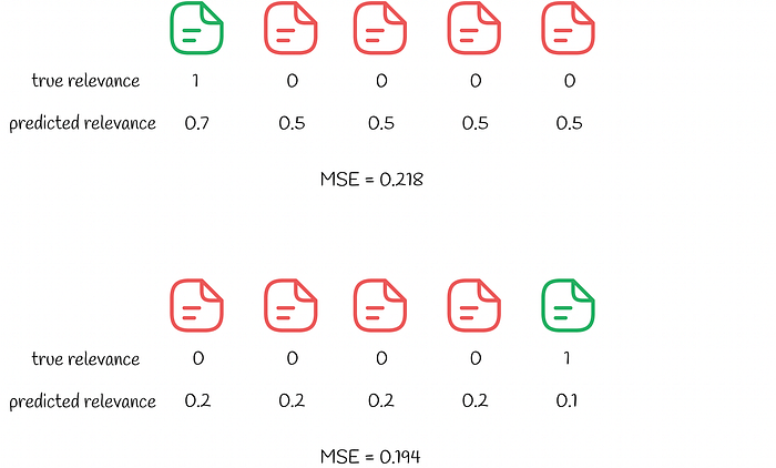 Error estimation for both queries shows that MSE is a bad metric for ranking. Green documents are relevant while red documents are irrelevant. The list of documents is shown in the order of predicted relevance (from left to right).
Though the second search result has a lower MSE, the user will not be satisfied with such a recommendation. By first looking only at non-relevant items, the user will have to scroll up all the way down to find the first relevant item. That is why from the user experience perspective, the first search result is much better: the user is just happy with the top item and proceeds to it while not caring about others. (View Highlight)
Error estimation for both queries shows that MSE is a bad metric for ranking. Green documents are relevant while red documents are irrelevant. The list of documents is shown in the order of predicted relevance (from left to right).
Though the second search result has a lower MSE, the user will not be satisfied with such a recommendation. By first looking only at non-relevant items, the user will have to scroll up all the way down to find the first relevant item. That is why from the user experience perspective, the first search result is much better: the user is just happy with the top item and proceeds to it while not caring about others. (View Highlight)- The same logic goes with classification metrics (precision, recall) which consider all items as well.
 Precision and recall formulas
What do all of described metrics have in common? All of them treat all items equally and do not consider any differentiation between high and low-relevant results. That is why they are called unranked. (View Highlight)
Precision and recall formulas
What do all of described metrics have in common? All of them treat all items equally and do not consider any differentiation between high and low-relevant results. That is why they are called unranked. (View Highlight) - Kendall Tau distance is based on the number of rank inversions.
An invertion is a pair of documents (i, j) such as document i having a greater relevance than document j, appears after on the search result than j. (View Highlight)
- Kendall Tau distance calculates all the number of inversions in the ranking. The lower the number of inversions, the better the search result is. Though the metric might look logical, it still has a downside which is demonstrated in the example below.
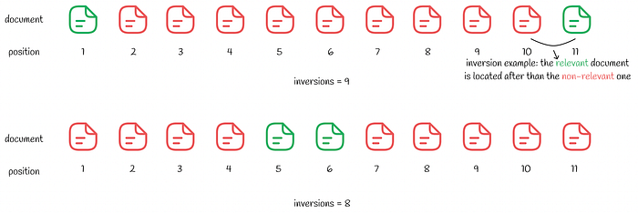 Despite fewer number of inversions, the second ranking is still worse, from the user perspective (View Highlight)
 - It seems like the second search result is better with only 8 inversions versus 9 in the first one. Similarly to the MSE example above, the user is only interested in the first relevant result. By going through several non-relevant search results in the second case, the user experience will be worse than in the first case. (View Highlight)
- Precision@k & Recall@k
Instead of usual precision and recall, it is possible to consider only at a certain number of top recommendations k. This way, the metric does not care about low-ranked results. Depending on the chosen value of k, the corresponding metrics are denoted as precision@k (“precision at k”) and recall@k (“recall at k”) respectively. Their formulas are shown below.
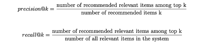 precision@k and recall@k formulas
Imagine top k results are shown to the user where each result can be relevant or not. precision@k measures the percentage of relevant results among top k results. At the same time, recall@k evaluates the ratio of relevant results among top k to the total number of relevant items in the whole dataset.
To better understand the calculation process of these metrics, let us refer to the example below.
precision@k and recall@k formulas
Imagine top k results are shown to the user where each result can be relevant or not. precision@k measures the percentage of relevant results among top k results. At the same time, recall@k evaluates the ratio of relevant results among top k to the total number of relevant items in the whole dataset.
To better understand the calculation process of these metrics, let us refer to the example below.
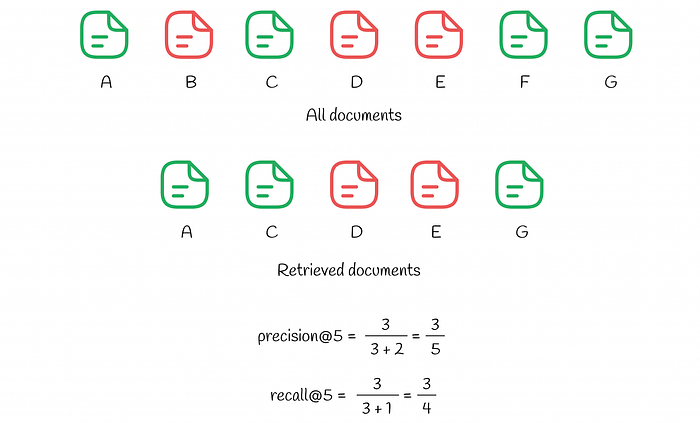 precision@k and recall@k calculation example. Green documents represent relevant items while the red ones correspond to irrelevant ones.
There are 7 documents in the system (named from A to G). Based on its predictions, the algorithm chooses k = 5 documents among them for the user. As we can notice, there are 3 relevant documents (A, C, G) among top k = 5 which results in precision@5 being equal to 3 / 5. At the same time, recall@5 takes into account relevant items in the whole dataset: there are 4 of them (A, C, F and G) making recall@5 = 3 / 4.
recall@k always increases with the growth of k making this metric not really objective in some scenarios. In the edge case where all the items in the system are shown to the user, the value of recall@k equals 100%. precision@k does not have the same monotonic property as recall@k has as it measures the ranking quality in relation to top k results, not in relation to the number of relevant items in the whole system. Objectivity is one of the reasons precision@k is usually a preferred metric over recall@k in practice. (View Highlight)
precision@k and recall@k calculation example. Green documents represent relevant items while the red ones correspond to irrelevant ones.
There are 7 documents in the system (named from A to G). Based on its predictions, the algorithm chooses k = 5 documents among them for the user. As we can notice, there are 3 relevant documents (A, C, G) among top k = 5 which results in precision@5 being equal to 3 / 5. At the same time, recall@5 takes into account relevant items in the whole dataset: there are 4 of them (A, C, F and G) making recall@5 = 3 / 4.
recall@k always increases with the growth of k making this metric not really objective in some scenarios. In the edge case where all the items in the system are shown to the user, the value of recall@k equals 100%. precision@k does not have the same monotonic property as recall@k has as it measures the ranking quality in relation to top k results, not in relation to the number of relevant items in the whole system. Objectivity is one of the reasons precision@k is usually a preferred metric over recall@k in practice. (View Highlight) - AP@k (Average Precision) & MAP@k (Mean Average Precision)
The problem with vanilla precision@k is that it does not take into account the order of relevant items appearing among retrieved documents. For example, if there are 10 retrieved documents with 2 of them being relevant, precision@10 will always be the same despite the location of these 2 documents among 10. For instance, if the relevant items are located in positions (1, 2) or (9, 10), the metric does differentiate both of these cases resulting in precision@10 being equal to 0.2.
However, in real life, the system should give a higher weight to relevant documents ranked on the top rather than on the bottom. This issue is solved by another metric called average precision (AP). As a normal precision, AP takes values between 0 and 1.
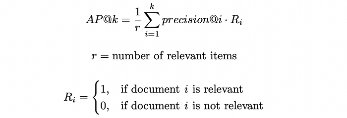 Average precision formula
AP@k calculates the average value of precision@i for all values of i from 1 to k for those of which the i-th document is relevant.
Average precision formula
AP@k calculates the average value of precision@i for all values of i from 1 to k for those of which the i-th document is relevant.
 Average precision computed for two queries (View Highlight)
 - In the figure above, we can see the same 7 documents. The response to the query Q₁ resulted in k = 5 retrieved documents where 3 relevant documents are positioned at indexes (1, 3, 4). For each of these positions i, precision@i is calculated: • precision@1 = 1 / 1 • precision@3 = 2 / 3 • precision@4 = 3 / 4 All other mismatched indexes i are ignored. The final value of AP@5 is computed as an average over the precisions above: • AP@5 = (precision@1 + precision@3 + precision@4) / 3 = 0.81 For comparison, let us look at the response to another query Q₂ which also contains 3 relevant documents among top k. Nevertheless, this time, 2 irrelevant documents are located higher in the top (at positions (1, 3)) than in the previous case which results in lower AP@5 being equal to 0.53. (View Highlight)
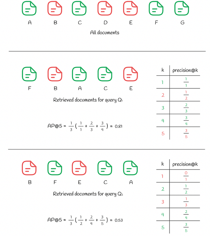
- Sometimes there is a need to evaluate the quality of the algorithm not on a single query but on multiple queries. For that purpose, the mean average precision (MAP) is utilised. Is is simply takes the mean of AP among several queries Q:
 Mean average precision formula
The example below shows how MAP is calculated for 3 different queries:
Mean average precision formula
The example below shows how MAP is calculated for 3 different queries:
 AP and MAP computed for three queries (View Highlight)
 - RR (Reciprocal Rank) & MRR (Mean Reciprocal Rank)
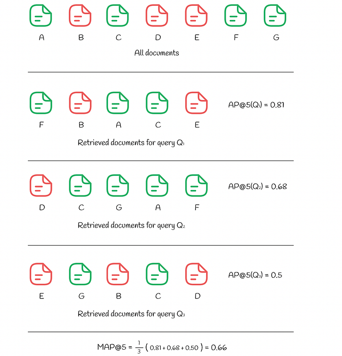
Sometimes users are interested only in the first relevant result. Reciprocal rank is a metric which returns a number between 0 and 1 indicating how far from the top the first relevant result is located: if the document is located at position k, then the value of RR is 1 / k.
Similarly to AP and MAP, mean reciprocal rank (MRR) measures the average RR among several queries.
 RR and MRR formulas
The example below shows how RR and MRR are computed for 3 queries:
RR and MRR formulas
The example below shows how RR and MRR are computed for 3 queries:
 RR and MRR computed for three queries (View Highlight)
 - User-oriented metrics
Though ranked metrics consider ranking positions of items thus being a preferable choice over the unranked ones, they still have a significant downside: the information about user behaviour is not taken into account.
User-oriented approaches make certain assumptions about user behaviour and based on it, produce metrics that suit ranking problems better.
DCG (Discounted Cumulative Gain) & nDCG (Normalized Discounted Cumulative Gain)
The DCG metric usage is based on the following assumption:
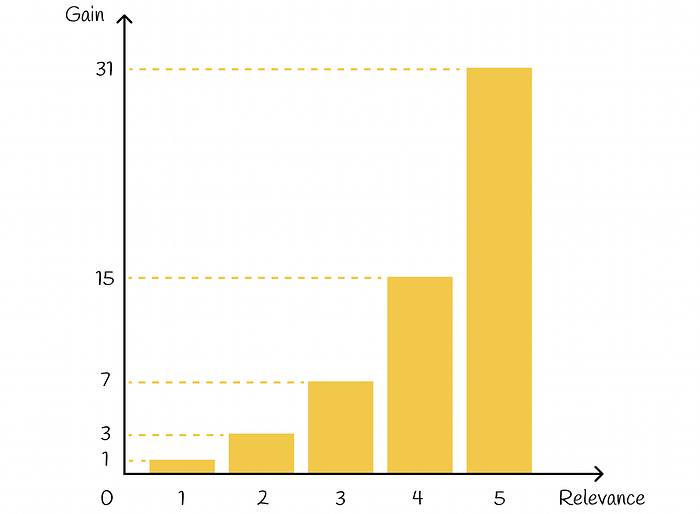
Highly relevant documents are more useful when appearing earlier in a search engine result list (have higher ranks) — Wikipedia This assumption naturally represents how users evaluate higher search results, compared to those presented lower. In DCG, each document is assigned a gain which indicates how relevant a particular document is. Given a true relevance Rᵢ (real value) for every item, there exist several ways to define a gain. One of the most popular is:
 Possible gain formula in DCG
Basically, the exponent puts a strong emphasis on relevant items. For example, if a rating of a movie is assigned an integer between 0 and 5, then each film with a corresponding rating will approximatively have double importance, compared to a film with the rating reduced by 1:
Possible gain formula in DCG
Basically, the exponent puts a strong emphasis on relevant items. For example, if a rating of a movie is assigned an integer between 0 and 5, then each film with a corresponding rating will approximatively have double importance, compared to a film with the rating reduced by 1:
 (View Highlight)
 - Apart from it, based on its ranking position, each item receives a discount value: the higher the ranking position of an item, the higher the corresponding discount is. Discount acts as a penalty by proportionally reducing the item’s gain. In practice, the discount is usually chosen as a logarithmic function of a ranking index:
 Discount formula in DCG
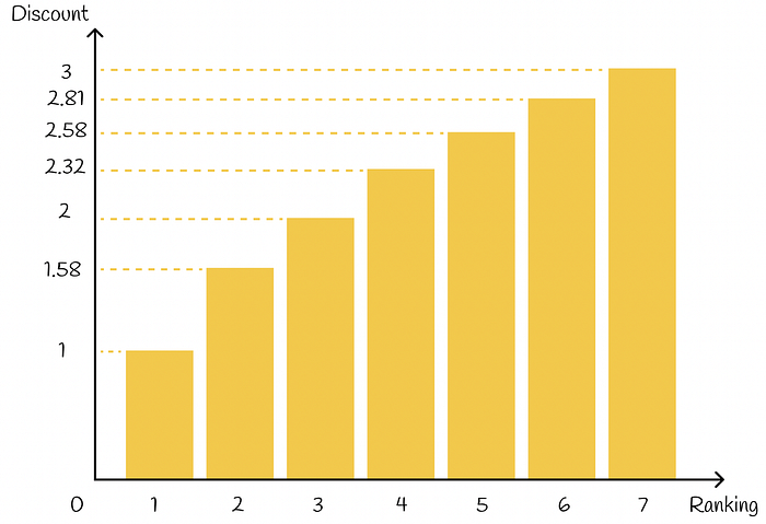 Discount function of ranking position
Finally, DCG@k is defined as the sum of a gain over a discount for all first k retrieved items:
Discount function of ranking position
Finally, DCG@k is defined as the sum of a gain over a discount for all first k retrieved items:
 DCG formula in general
Replacing gainᵢ and discountᵢ with the formulas above, the expression takes the following form:
DCG formula in general
Replacing gainᵢ and discountᵢ with the formulas above, the expression takes the following form:
 DCG formula (View Highlight)
 - To make DCG metric more interpretable, it is usually normalised by the maximum possible value of DCGₘₐₓ in the case of perfect ranking when all items are correctly sorted by their relevance. The resulting metric is called nDCG and takes values between 0 and 1.
 nDCG formula
In the figure below, an example of DCG and nDCG calculation for 5 documents is shown.
nDCG formula
In the figure below, an example of DCG and nDCG calculation for 5 documents is shown.
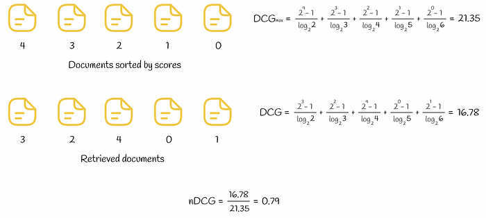 DCG and nDCG computed for a set of retrieved documents (View Highlight)
 - RBP (Rank-Biased Precision)
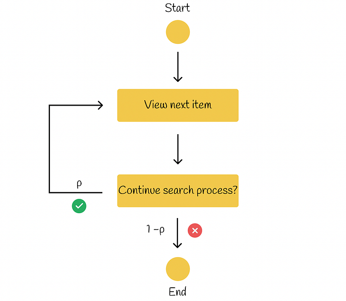
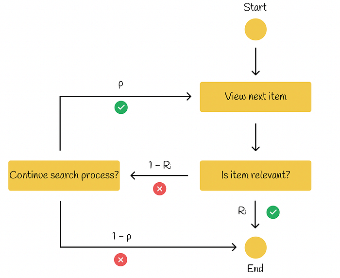
In the RBP workflow, the user does not have the intention to examine every possible item. Instead, he or she sequentially progresses from one document to another with probability p and with inverse probability 1 — p terminates the search procedure at the current document. Each termination decision is taken independently and does not depend on the depth of the search. According to the conducted research, such user behaviour has been observed in many experiments. Based on the information from Rank-Biased Precision for Measurement of Retrieval Effectiveness, the workflow can be illustrated in the diagram below.
Parameter p is called persistence.
 RBP model workflow
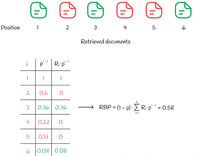
In this paradigm, the user looks always looks at the 1-st document, then looks at the 2-nd document with probability p, looks at the 3-rd document with probability p² and so on. Ultimately, the probability of looking at document i becomes equal to:
RBP model workflow
In this paradigm, the user looks always looks at the 1-st document, then looks at the 2-nd document with probability p, looks at the 3-rd document with probability p² and so on. Ultimately, the probability of looking at document i becomes equal to:
 The user examines document i in only when document i has just already been looked at and the search procedure is immediately terminated with probability 1 — p.
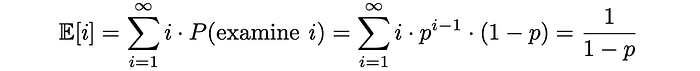
 After that, it is possible to estimate the expected number of examined documents. Since 0 ≤ p ≤ 1, the series below is convergent and the expression can be transformed into the following format:
 Similarly, given each document’s relevance Rᵢ, let us find the expected document relevance. Higher values of expected relevance indicate that the user will be more satisfied with the document he or she decides to examine.
 Finally, RPB is computed as the ratio of expected document relevance (utility) to the expected number of checked documents:
 RPB formulation makes sure that it takes values between 0 and 1. Normally, relevance scores are of binary type (1 if a document is relevant, 0 otherwise) but can take real values between 0 and 1 as well.
The appropriate value of p should be chosen, based on how persistent users are in the system. Small values of p (less than 0.5) place more emphasis on top-ranked documents in the ranking. With bigger values of p, the weight on first positions is reduced and is distributed across lower positions. Sometimes it might be difficult to find out a good value of persistence p, so it is better to run several experiments and choose p which works the best.
RPB formulation makes sure that it takes values between 0 and 1. Normally, relevance scores are of binary type (1 if a document is relevant, 0 otherwise) but can take real values between 0 and 1 as well.
The appropriate value of p should be chosen, based on how persistent users are in the system. Small values of p (less than 0.5) place more emphasis on top-ranked documents in the ranking. With bigger values of p, the weight on first positions is reduced and is distributed across lower positions. Sometimes it might be difficult to find out a good value of persistence p, so it is better to run several experiments and choose p which works the best.
 (View Highlight)
 - ERR (Expected Reciprocal Rank)
As the name suggests, this metric measures the average reciprocal rank across many queries.
This model is similar to RPB but with a little difference: if the current item is relevant (Rᵢ) for the user, then the search procedure ends. Otherwise, if the item is not relevant (1 — Rᵢ), then with probability p the user decides whether he or she wants to continue the search process. If so, the search proceeds to the next item. Otherwise, the users ends the search procedure.
 ERR model workflow
According to the presentation on offline evaluation from Ilya Markov, let us find the formula for ERR calculation. (View Highlight)
ERR model workflow
According to the presentation on offline evaluation from Ilya Markov, let us find the formula for ERR calculation. (View Highlight) - We have discussed all the main metrics used for quality evaluation in information retrieval. User-oriented metrics are used more often because they reflect real user behaviour. Additionally, nDCG, BPR and ERR metrics have an advantage over other metrics we have looked at so far: they work with multiple relevance levels making them more versatile, in comparison to metrics like AP, MAP or MRR which are designed only for binary levels of relevance. (View Highlight)