Learning with not Enough Data Part 3: Data Generation

Metadata §

• Author: Lilian Weng
• Full Title: Learning with not Enough Data Part 3: Data Generation
• URL: https://lilianweng.github.io/posts/2022-04-15-data-gen/

Highlights §

• Let’s consider two approaches for generating synthetic data for training. • Augmented data. Given a set of existing training samples, we can apply a variety of augmentation, distortion and transformation to derive new data points without losing the key attributes. We have covered a bunch of augmentation methods on text and images in a previous post on contrastive learning. For the sake of post completeness, I duplicate the section on data augmentation here with some edits. • New data. Given few or even no data points, we can rely on powerful pretrained models to generate a number of new data points. This is especially true in recent years given the fast progress in large pretrained language models (LM). Few shot prompting is shown to be effective for LM to learn within context without extra training. (View Highlight)
• Image Augmentation#Basic Image Processing Operations# There are several ways to modify an image while retaining its semantic information. We can use any one of the following augmentation or a composition of multiple operations. • Random cropping and then resize back to the original size. • Random color distortions • Random Gaussian blur • Random color jittering • Random horizontal flip • Random grayscale conversion • And many more. Check PIL.ImageOps for inspiration. (View Highlight)
• Task-Specific Augmentation Strategies# If the downstream task is known, it is possible to learn the optimal augmentation strategies (i.e. what processing operations to use and how to combine them in sequence) to maximize the downstream task performance. • AutoAugment (Cubuk, et al. 2018) is inspired by neural architecture search, AutoAugment frames the problem of learning best data augmentation operations (i.e. shearing, rotation, invert, etc.) for image classification as an RL problem and looks for the combination that leads to the highest accuracy on the evaluation set. AutoAugment can be executed in adversarial fashion (Zhang, et al 2019). • RandAugment (Cubuk et al., 2019) greatly reduces the search space of AutoAugment by controlling the magnitudes of different transformation operations with a single magnitude parameter. • Population based augmentation (PBA; Ho et al., 2019) combines PBT (“population based training”; Jaderberg et al, 2017) with AutoAugment, using the evolutionary algorithm to train a population of children models in parallel to evolve the best augmentation strategies. • Unsupervised Data Augmentation (UDA; Xie et al., 2019), among a set of possible augmentation strategies, selects a subset to minimize the KL divergence between the predicted distribution over an unlabelled example and its unlabelled augmented version. (View Highlight)
• Image Mixture# Image mixture methods can construct new training examples from existing data points. (View Highlight)
• Text Augmentation#Lexical Edits# Easy Data Augmentation (EDA; Wei & Zou 2019) defines a set of simple but powerful operations for text augmentation. Given a sentence, EDA randomly chooses and applies one of four simple operations:
  1. Synonym replacement (SR): Replace n random non-stop words with their synonyms.
  2. Random insertion (RI): Place a random synonym of a randomly selected non-stop word in the sentence at a random position.
  3. Random swap (RS): Randomly swap two words and repeat n times.
  4. Random deletion (RD): Randomly delete each word in the sentence with probability p. where p=α and n=α×sentence_length, with the intuition that longer sentences can absorb more noise while maintaining the original label. The hyperparameter α roughly indicates the percent of words in one sentence that may be changed by one augmentation. EDA is shown to improve the classification accuracy on several classification benchmark datasets compared to baseline without EDA. The performance lift is more significant on a smaller training set. (View Highlight)
• Contextual Augmentation (Kobayashi, 2018) replaces word wi at position i by sampling from a probability distribution learned by a bidirectional LM such as BERT, p(.∣S∖wi). In this way, the words are substituted by synonyms, or similar words suitable for the context. To guarantee such operations do not alter the labels, the LM is fit to be label-conditioned bidirectional LM. Conditional BERT (CBERT; Xing Wu et al. 2018) extends BERT to predict masked tokens conditioned on the class label and can be used for contextual augmentation prediction. (View Highlight)
• Back-translation# Back-translation produces augmented data by translating text samples to another language and then translating them back. The translation happens in two ways and both directions should have decent enough performance to avoid significant loss of semantic meaning. (View Highlight)
• Mix-up# It is also possible to apply Mixup to text (Guo et al. 2019) but on the embedding space to obtain some performance gain. The proposed method relies on a specially designed model architecture to operate the prediction on the word or sentence embedding. Adding adversarial noise in the embedding space as a way of data augmentation is shown to improve the generalization of model training (Zhu et al. 2019). (View Highlight)
• Given that generating high-quality, photorealistic images is a lot more difficult than generating human-like natural language text and recent success with large pretrained language models, this section only focuses on text generation. (View Highlight)
• Language Model as Noisy Annotator# Wang et al. (2021) explored ways to leverage GPT-3 as a weak annotator via few-shot prompting, achieving 10x cheaper than human labeling. The paper argues that by using data labeled by GPT-3, it essentially performs self-training: The predictions on unlabeled samples apply entropy regularization on the model to avoid high class overlaps so as to help improve the model performance. 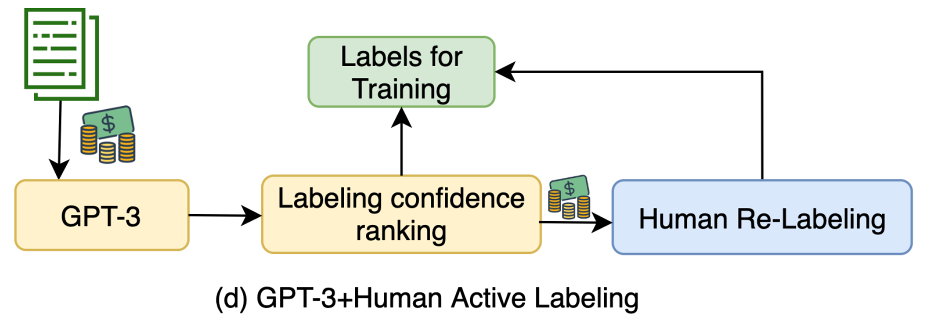Fig. 2. Illustration of how to use GPT-3 to generate more training data with the human-in-the-loop active learning pipeline to improve the data quality. (Image source: Wang et al. 2021) GPT-3-labeled samples selected by active learning with highest uncertainty are sent to human labelers to be re-annotated. The few-shot prompt contains a small number of human labeled examples and thus the labeling cost is restricted. Synthetic samples are ranked by predicted logits of label y and those with the lowest scores go through relabeling. GPT-3 labeling achieves better results in the low-cost regime, but has a gap with human labeling when enough money is spent on data collection. This implies the following inequation, although to what extent “a lot” or “noisy” means depends on the task details.

  A lot of high-quality data > A lot of noisy data > A little high quality data. (View Highlight)

• Language Model as Data Generator# If enough training dataset for text classification tasks are available, we can fine-tune language models to synthesize more training samples conditioned on labels (Anaby-Tavor et al. 2019, Kumar et al. 2021). Language-model-based data augmentation (LAMBADA; Anaby-Tavor et al. 2019) takes such an idea, where the process involves fine-tuning both a classifier and a sample generation model.
  1. Train a baseline classifier using the existing training dataset: h=A(Dtrain).
  2. Independently of step 1, a LM M is fine-tuned on Dtrain to obtain Mtuned.
  3. Synthesize a labeled dataset D∗ by generating the continuation of the sequence y[SEP] until EOS using Mtuned.
  4. Filter synthesized dataset by, • (1) Verifying that the predicted label is correct h(x)=y; • (2) Selecting the top ranked samples when they are ranked by the classifier probability. Dsyn⊂D∗. They generate 10x more samples needed for augmentation and only the top 10% synthesized samples with highest confidence scores remain. (View Highlight)
• To simplify LAMBADA, we can actually remove the dependency of a fine-tuned generation model and an existing training dataset of a decent size (Step 2 above). Unsupervised data generation (UDG; Wang et al. 2021) relies on few-shot prompting on a large pretrained language model to generate high-quality synthetic data for training. Opposite to the above approach where LM is asked to predict y given x, UDG instead synthetizes the inputs x given labels y. Then a task-specific model is trained on this synthetic dataset. (View Highlight)
• Schick & Schutze (2021) proposed a similar idea but on the NLI task instead of classification, asking PLM to write sentence pairs that are similar or different while the model is prompted with task-specific instructions. 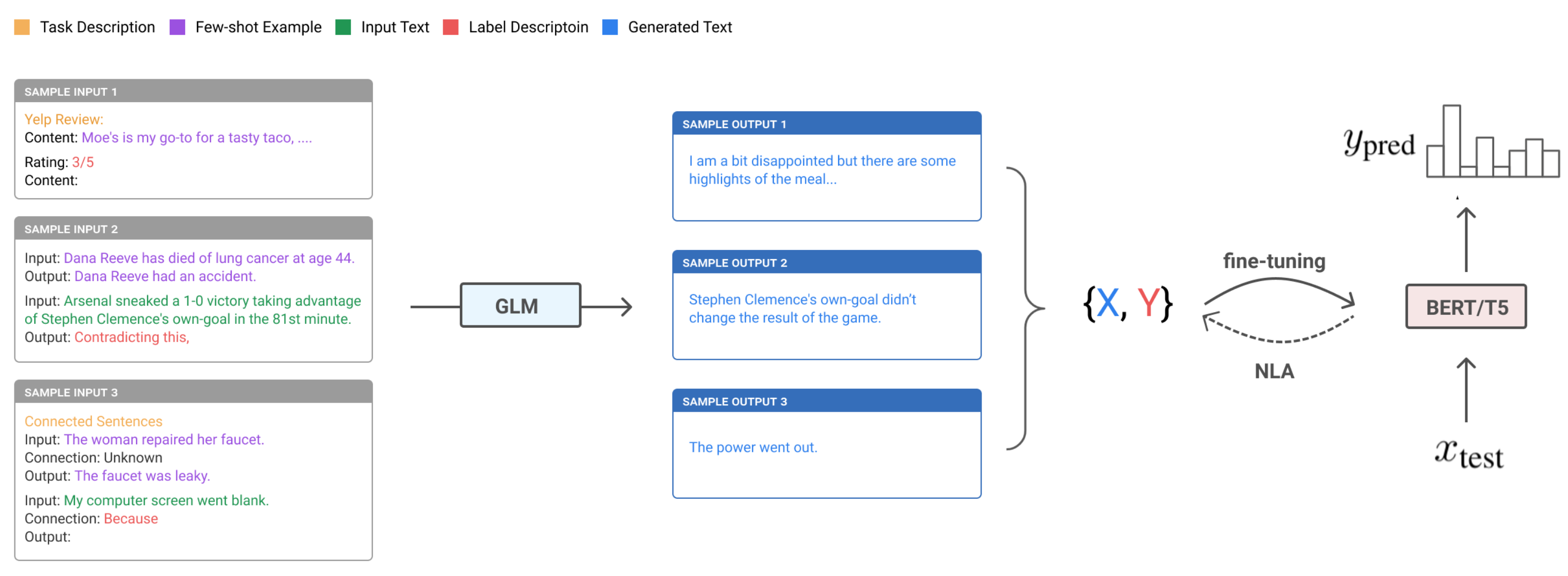Fig. 5. Illustration of the unsupervised data generation (UDG) framework. (Image source: Wang et al., 2021) (View Highlight)
• The few-shot prompts of UDG contain a small number of unlabeled examples, as well as a task-specific natural language description of the desired label. Because some generated examples are noisy, they implemented noisy label annealing (NLA) techniques to filter potentially misaligned samples out during the training processes. NLA gradually removes noisy training signals in time during training when the model starts to disagree with its pseudo label with high confidence. At each training step t, a given example (xi,y^i) is considered noisy and should be removed if: • The model predicted probability is higher than a threshold p(y¯i|xi)>μt where y¯i=arg⁡maxyp(y|xi); • And the predicted label is different from the synthetic label, y¯i≠y^i. Note that the threshold μt is time-dependent, initialized as 0.9 and then gradually annealed to 1/num_of_classes in time. As shown in their experiments, the improvement of UDG over few-shot inference is quit significant, where NLA brings in some extra boost. The results are even comparable with supervised fine-tuning on several cases. (View Highlight)
• Han et al (2021) achieved SOTA results on translation tasks using few-shot data generation, distillation and back-translation. The proposed method contains the following steps, assuming no access to paired translation data:
  1. Zero-shot Generation. First use the zero-shot translation ability of a pre-trained LM to generate translations for a small set of unlabeled sentences.
  2. Few-shot Generation. Then amplify these zero-shot translations by using them as few-shot demonstrations to gather an even larger synthetic dataset.
  3. Distillation. Fine-tune the model on this dataset. The translation task is formulated as a language modeling task [L1] <seq1> [[TRANSLATE]] [L2] <seq2>. given a pair of two sequences <seq1, seq2> in two different languages. At test-time, the LM is prompted with [L1] <seq> [[TRANSLATE]] [L2] and a candidate translation <sampledSeq> is parsed from the sampled completion.
  4. Back-translation. Continue fine-tuning on the back-translation dataset where the order of samples is reversed, <sampledSeq, seq>.
  5. Step 1-4 can be repeated. (View Highlight)
• The success of the above method depends on a good pretrained LM to kick off the initial translation dataset. Iterative few-shot generation and distillation with back-translation is an effective way to extract and refine the translation capability out of a pretrained LM and further to distill that into a new model. 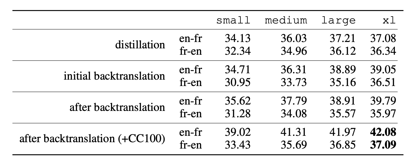Fig. 8. Comparison of BLEU scores of the translation models of different training runs using: only distillation, back-translation, both and with more monolingual training data. (Image source: Han et al. 2021) (View Highlight)
• Given all the generated data, either by data augmentation or data synthesis, how can we quantify data quality in terms of how they improve model generalization? Gontijo-Lopes et al. (2020) introduced two dimensions to track, affinity and diversity. • Affinity is a model-sensitive metric for distribution shift, quantifying how much an augmentation shifts the training data distribution from what a model learned. • Definition: The performance difference between the model tested on clean data vs augmented data, while the model is trained on clean data. • As a comparison, KL can also measure distribution shift but does not consider the model performance. • Diversity is a measure of augmentation complexity, measuring the complexity of the augmented data with respect to the model and learning procedure. • Definition: The final training loss of a model trained with a given augmentation. • Another potential diversity measure is the entropy of the transformed data. • A third potential diversity measure is the training time needed for a model to reach a given training accuracy threshold. • All three metrics above are correlated. The final model performance is dependent on both metrics to be high enough. 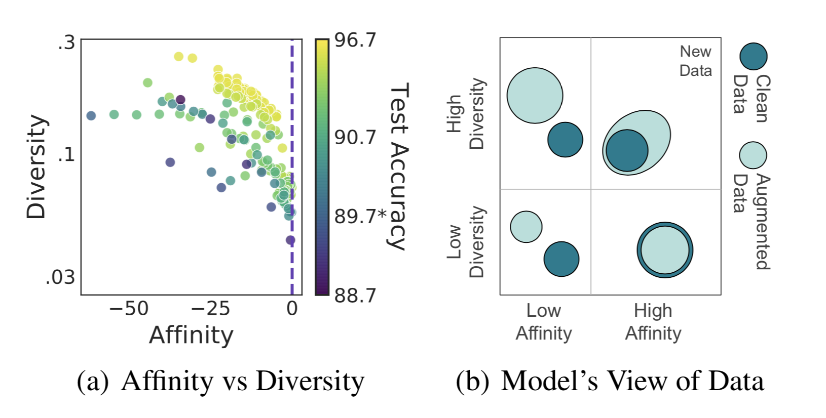Fig. 9. (a) Left: A scatter plot of affinity vs diversity metric, where each point represents a different augmentation method and its color indicates the final test accuracy. (b) Right: The conceptual illustration of the relationship between clean and augmented data in different regions of affinity and diversity metrics. (Image source: Gontijo-Lopes et al. 2020) There are many quantitative metrics on relevancy and diversity, in different formations depending on whether a reference is available, such as perplexity, BLEU for text and inception score for images. I’m skipping the list of concrete quantitative metrics on quality here, given it could be very long. (View Highlight)
• Training with Noisy Data# It is convenient to collect a large amount of noisy data via model generation or data augmentation, but it is hard to guarantee that augmented and generated data can be 100% accurate. Knowing that deep neural networks can easily overfit noisy labels and “memotize” corrupted labels, we can apply the techniques for training on noisy labels (noise-robust training) when using generated data to stabilize and optimize the performance. (View Highlight)
• Regularization and Robust Architecture# Generally speaking, mechanisms designed for avoiding overfitting should help improve training robustness when working with moderately noisy data, such as weight decay, dropout, batch normalization. In fact, good data augmentation (i.e. only non-essential attributes are modified) can be considered as a way of regularization as well. A different approach is to enhance the network with a dedicated noisy adaptation layer to approximate the unknown projection of label corruption (Sukhbaatar et al. 2015, Goldberger & Ben-Reuven, 2017). Sukhbaatar et al. (2015) introduced an extra linear layer Q into the network architecture to adapt the predictions to match the noisy label distribution. The noise matrix Q is initially fixed to the identity function while only the base model parameters is updated. After some time, Q starts to be updated and expected to capture the noise in the data. The noise matrix is trained with regularization to encourage it to match the noise distribution while keeping the base model prediction accurate for true labels. 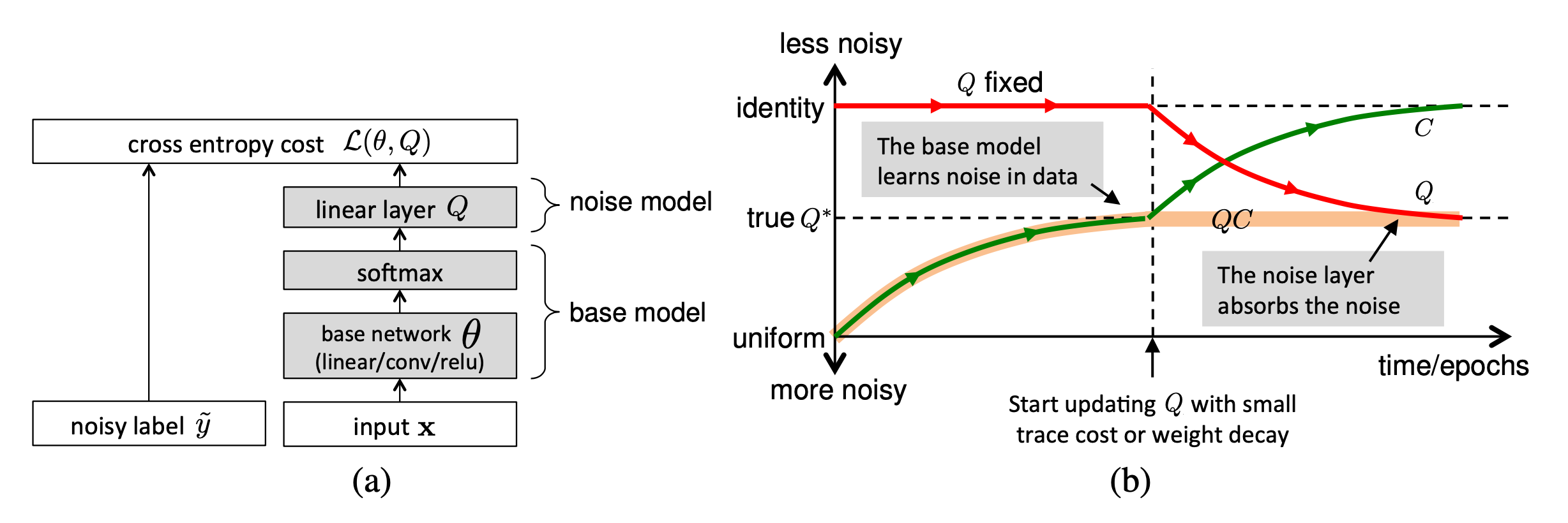Fig. 10. (a) Left: A noise matrix Q is added between softmax and the final output for the loss. (b) Right: The noise matrix Q is fixed at the identity function initially and only gets updated with regularization after some training. (Image source: Sukhbaatar et al. 2015) However, it is hard to guarantee such a noise matrix layer would only capture the noise transition distribution and it is actually non-trivial to learn. Goldberger & Ben-Reuven (2017)) proposed to add an additional softmax layer end-to-end with the base model and apply the EM algorithm by treating the correct labels as latent random variable and the noise processes as a communication channel with unknown parameters. (View Highlight)
• Robust Learning Objective# Besides the most commonly used cross entropy loss, some other choices of learning objectives are shown to be more robust to noisy labels. For example, MAE (mean absolute error) is more robust to noisy labels than CCE (categorical cross entropy), as it treats every sample equally (Ghosh et al. 2017). Lack of different weighting among training samples of MAE lead to significantly longer training time. Motivated by the tradeoff between MAE and CCE, Zhang & Sabuncu (2018) proposed generalized cross entropy (GCE), a generalization of CCE loss to be robust to noisy data. To exploit the benefits of both the noise-robustness provided by MAE and the implicit weighting scheme of CCE, GCE adopts the the negative Box-Cox transformation as a loss function (View Highlight)
• Label Correction# Since it is known some labels are incorrect, noise-robust training can explicitly take the label correction into consideration. One approach is to rely on the estimation of a noise transition matrix and use that to correct the forward or backward loss, named F-correction (Patrini et al. 2017). (View Highlight)
• Sample Reweighting and Selection# Some samples may be more likely to have inaccurate labels than others. Such estimation gives us intuition on which samples should be weighted less or more in the loss function. However, considering two types of biases in training data, class imbalance and noisy labels, there is actually a contradictory preference — We would prefer samples with larger loss to balance the label distribution but those with smaller loss for mitigating the potential noise. Some work (Ren et al. 2018) thus argue that in order to learn general forms of training data biases, it is necessary to have a small unbiased validation to guide training. The sample reweighting methods presented in this section all assume access to a small trusted set of clean data. (View Highlight)
• MentorNet (Jiang et al. 2018) uses teach-student curriculum learning to weight data. It incorporates two different networks, a mentor and a student. The mentor network provides a data-driven curriculum (i.e. sample training weighting scheme) for the student to focus on learning likely correct labels. (View Highlight)