
Highlights §
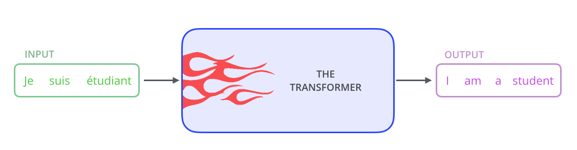
- we will look at The Transformer – a model that uses attention to boost the speed with which these models can be trained. (View Highlight)
 (View Highlight)
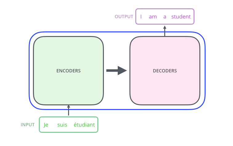 (View Highlight)
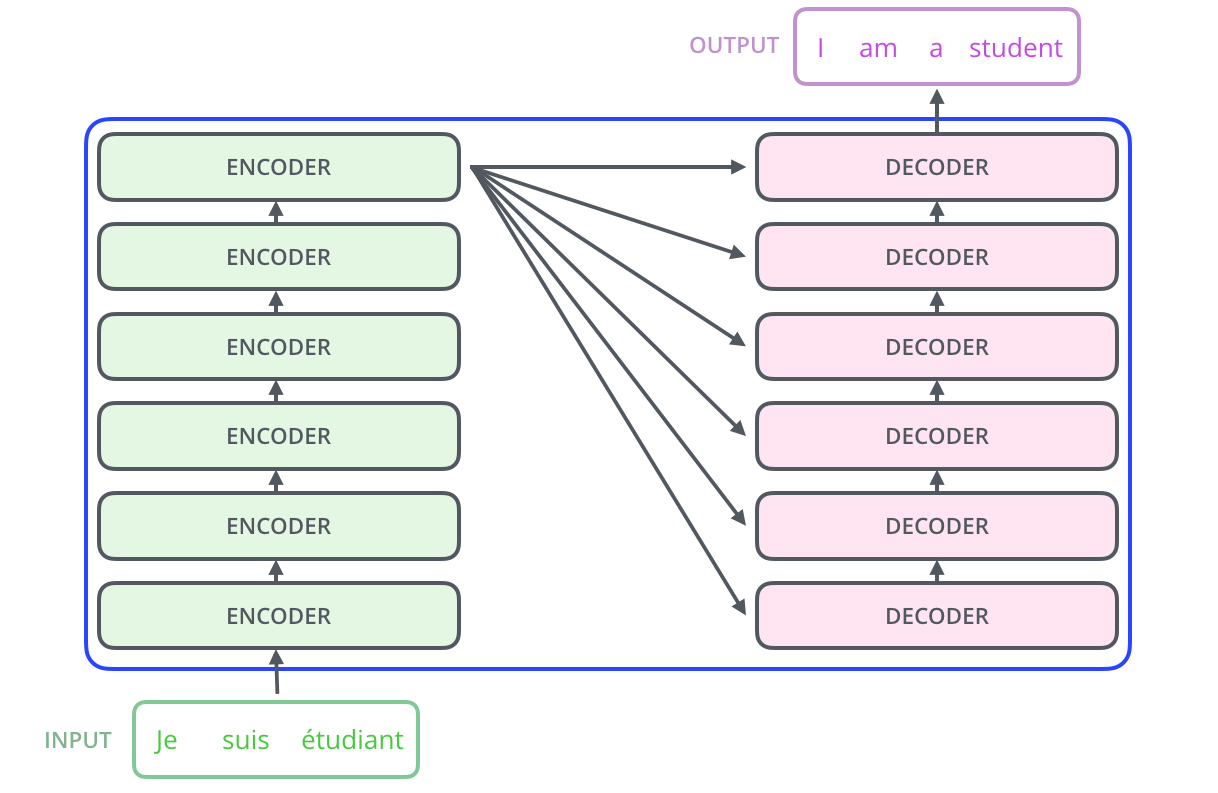
- The encoding component is a stack of encoders (the paper stacks six of them on top of each other – there’s nothing magical about the number six, one can definitely experiment with other arrangements). The decoding component is a stack of decoders of the same number. (View Highlight)
 (View Highlight)
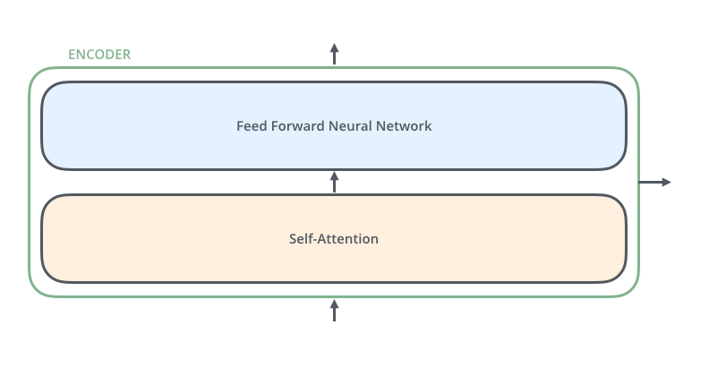
- The encoders are all identical in structure (yet they do not share weights). Each one is broken down into two sub-layers: (View Highlight)
 (View Highlight)
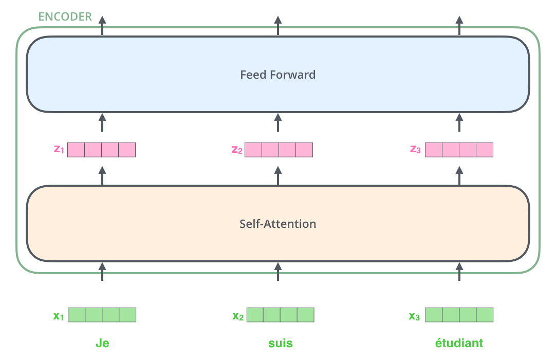
- The encoder’s inputs first flow through a self-attention layer – a layer that helps the encoder look at other words in the input sentence as it encodes a specific word. (View Highlight)
- The outputs of the self-attention layer are fed to a feed-forward neural network. The exact same feed-forward network is independently applied to each position. (View Highlight)
- The decoder has both those layers, but between them is an attention layer that helps the decoder focus on relevant parts of the input sentence (similar what attention does in seq2seq models). (View Highlight)
- As is the case in NLP applications in general, we begin by turning each input word into a vector using an embedding algorithm. (View Highlight)
- The embedding only happens in the bottom-most encoder. The abstraction that is common to all the encoders is that they receive a list of vectors each of the size 512 – In the bottom encoder that would be the word embeddings, but in other encoders, it would be the output of the encoder that’s directly below (View Highlight)
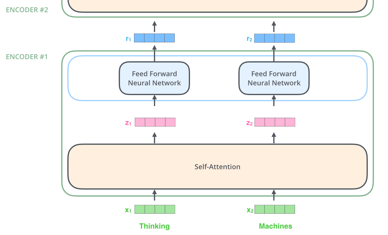
- After embedding the words in our input sequence, each of them flows through each of the two layers of the encoder. (View Highlight)
 (View Highlight)
- Here we begin to see one key property of the Transformer, which is that the word in each position flows through its own path in the encoder. There are dependencies between these paths in the self-attention layer. The feed-forward layer does not have those dependencies, however, and thus the various paths can be executed in parallel while flowing through the feed-forward layer. (View Highlight)
- an encoder receives a list of vectors as input. It processes this list by passing these vectors into a ‘self-attention’ layer, then into a feed-forward neural network, then sends out the output upwards to the next encoder. (View Highlight)
 (View Highlight)
- Don’t be fooled by me throwing around the word “self-attention” like it’s a concept everyone should be familiar with. I had personally never came across the concept until reading the Attention is All You Need paper. Let us distill how it works.
Say the following sentence is an input sentence we want to translate:
”
The animal didn't cross the street because it was too tired”
What does “it” in this sentence refer to? Is it referring to the street or to the animal? It’s a simple question to a human, but not as simple to an algorithm. (View Highlight)
- When the model is processing the word “it”, self-attention allows it to associate “it” with “animal”. (View Highlight)
- As the model processes each word (each position in the input sequence), self attention allows it to look at other positions in the input sequence for clues that can help lead to a better encoding for this word. (View Highlight)
- If you’re familiar with RNNs, think of how maintaining a hidden state allows an RNN to incorporate its representation of previous words/vectors it has processed with the current one it’s processing. Self-attention is the method the Transformer uses to bake the “understanding” of other relevant words into the one we’re currently processing. (View Highlight)
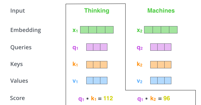
- The first step in calculating self-attention is to create three vectors from each of the encoder’s input vectors (in this case, the embedding of each word). So for each word, we create a Query vector, a Key vector, and a Value vector. These vectors are created by multiplying the embedding by three matrices that we trained during the training process. (View Highlight)
- Notice that these new vectors are smaller in dimension than the embedding vector. Their dimensionality is 64, while the embedding and encoder input/output vectors have dimensionality of 512. They don’t HAVE to be smaller, this is an architecture choice to make the computation of multiheaded attention (mostly) constant. (View Highlight)
- What are the “query”, “key”, and “value” vectors?
They’re abstractions that are useful for calculating and thinking about attention. Once you proceed with reading how attention is calculated below, you’ll know pretty much all you need to know about the role each of these vectors plays.
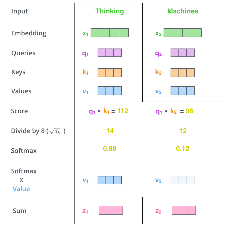
The second step in calculating self-attention is to calculate a score. Say we’re calculating the self-attention for the first word in this example, “Thinking”. We need to score each word of the input sentence against this word. The score determines how much focus to place on other parts of the input sentence as we encode a word at a certain position. (View Highlight)
- The score is calculated by taking the dot product of the query vector with the key vector of the respective word we’re scoring. So if we’re processing the self-attention for the word in position #1, the first score would be the dot product of q1 and k1. The second score would be the dot product of q1 and k2. (View Highlight)
 (View Highlight)
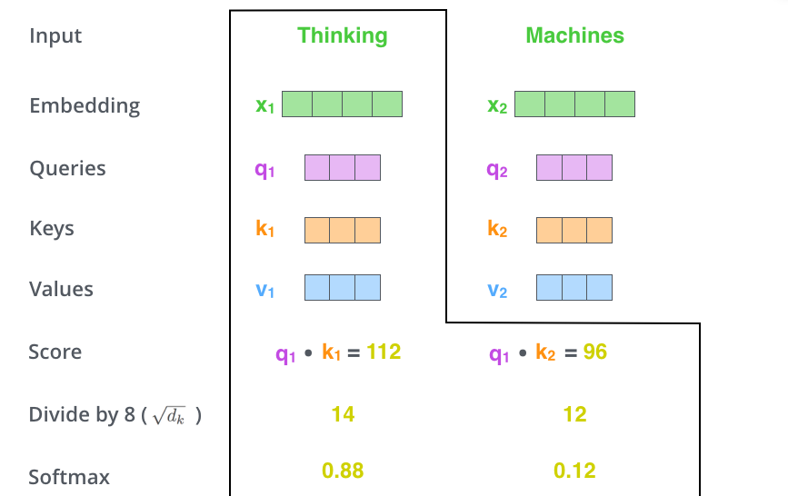
- The third and fourth steps are to divide the scores by 8 (the square root of the dimension of the key vectors used in the paper – 64. This leads to having more stable gradients. There could be other possible values here, but this is the default), then pass the result through a softmax operation. Softmax normalizes the scores so they’re all positive and add up to 1. (View Highlight)
 (View Highlight)
- his softmax score determines how much each word will be expressed at this position. Clearly the word at this position will have the highest softmax score, but sometimes it’s useful to attend to another word that is relevant to the current word. (View Highlight)
- The fifth step is to multiply each value vector by the softmax score (in preparation to sum them up). The intuition here is to keep intact the values of the word(s) we want to focus on, and drown-out irrelevant words (by multiplying them by tiny numbers like 0.001, for example) (View Highlight)
- The sixth step is to sum up the weighted value vectors. This produces the output of the self-attention layer at this position (for the first word). (View Highlight)
 (View Highlight)
- That concludes the self-attention calculation. The resulting vector is one we can send along to the feed-forward neural network. In the actual implementation, however, this calculation is done in matrix form for faster processing. So let’s look at that now that we’ve seen the intuition of the calculation on the word level. (View Highlight)
- Matrix Calculation of Self-Attention
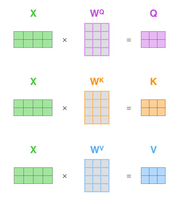
The first step is to calculate the Query, Key, and Value matrices. We do that by packing our embeddings into a matrix X, and multiplying it by the weight matrices we’ve trained (WQ, WK, WV). (View Highlight)
 (View Highlight)
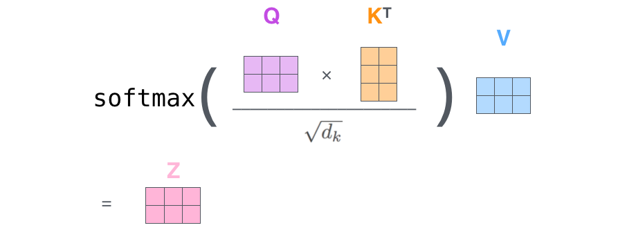
- Finally, since we’re dealing with matrices, we can condense steps two through six in one formula to calculate the outputs of the self-attention layer.
 (View Highlight)
- The paper further refined the self-attention layer by adding a mechanism called “multi-headed” attention. This improves the performance of the attention layer in two ways:
- It expands the model’s ability to focus on different positions. Yes, in the example above, z1 contains a little bit of every other encoding, but it could be dominated by the actual word itself. If we’re translating a sentence like “The animal didn’t cross the street because it was too tired”, it would be useful to know which word “it” refers to. (View Highlight)
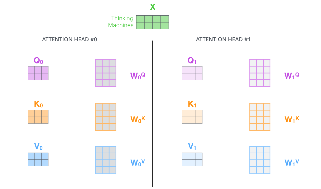
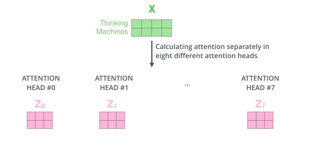
- It gives the attention layer multiple “representation subspaces”. As we’ll see next, with multi-headed attention we have not only one, but multiple sets of Query/Key/Value weight matrices (the Transformer uses eight attention heads, so we end up with eight sets for each encoder/decoder). Each of these sets is randomly initialized. Then, after training, each set is used to project the input embeddings (or vectors from lower encoders/decoders) into a different representation subspace. (View Highlight)
 (View Highlight)
- f we do the same self-attention calculation we outlined above, just eight different times with different weight matrices, we end up with eight different Z matrices
 (View Highlight)
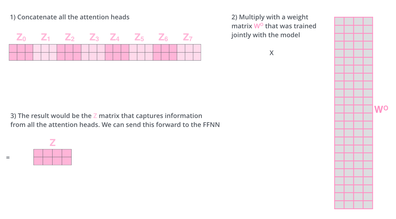
- This leaves us with a bit of a challenge. The feed-forward layer is not expecting eight matrices – it’s expecting a single matrix (a vector for each word). So we need a way to condense these eight down into a single matrix.
How do we do that? We concat the matrices then multiply them by an additional weights matrix WO.
 (View Highlight)
- That’s pretty much all there is to multi-headed self-attention. It’s quite a handful of matrices, I realize. Let me try to put them all in one visual so we can look at them in one place (View Highlight)
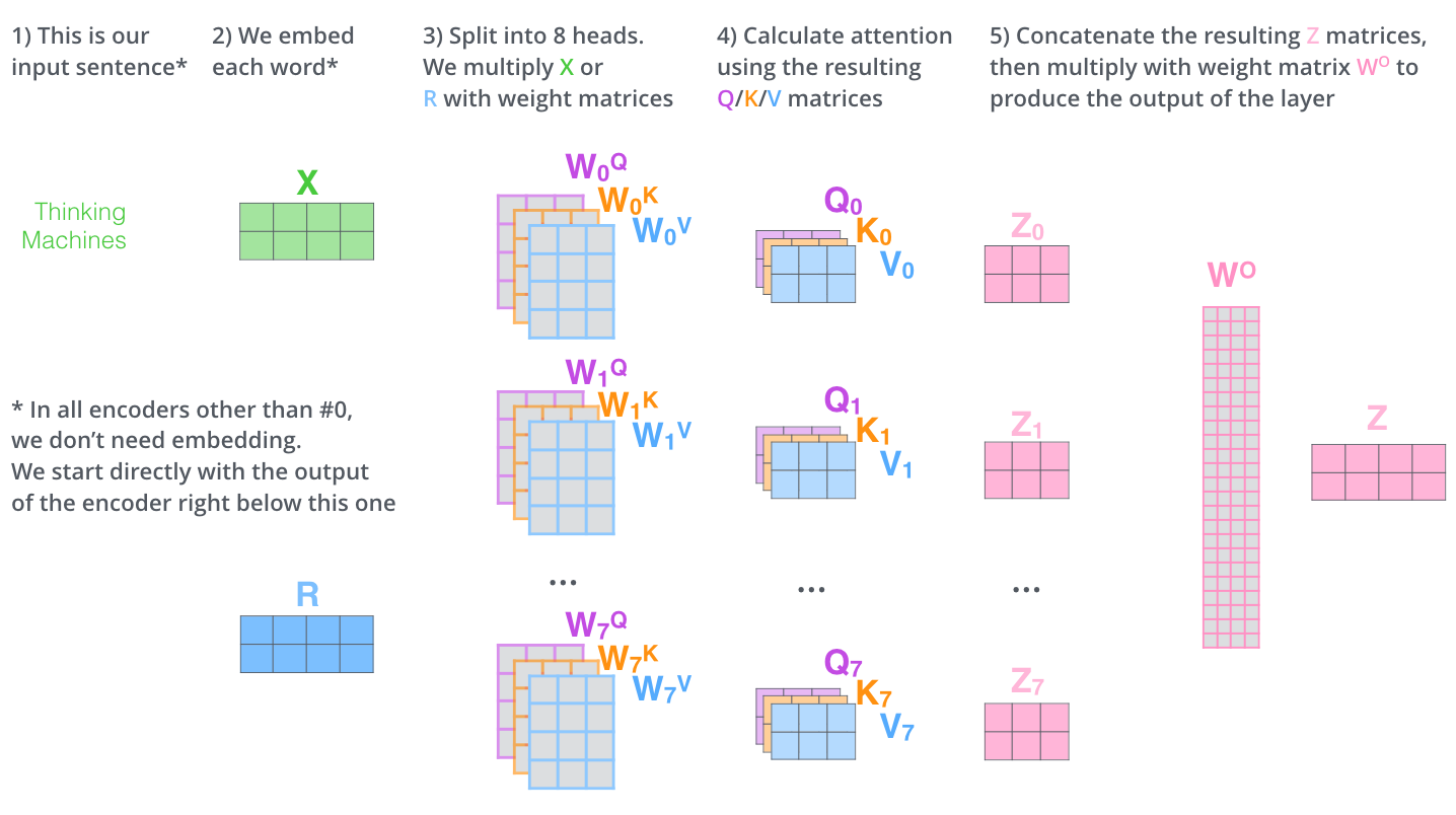 (View Highlight)
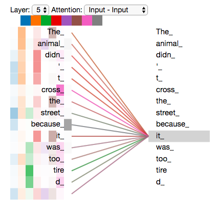
- Now that we have touched upon attention heads, let’s revisit our example from before to see where the different attention heads are focusing as we encode the word “it” in our example sentence:
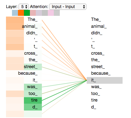 As we encode the word “it”, one attention head is focusing most on “the animal”, while another is focusing on “tired” — in a sense, the model’s representation of the word “it” bakes in some of the representation of both “animal” and “tired”.
If we add all the attention heads to the picture, however, things can be harder to interpret:
As we encode the word “it”, one attention head is focusing most on “the animal”, while another is focusing on “tired” — in a sense, the model’s representation of the word “it” bakes in some of the representation of both “animal” and “tired”.
If we add all the attention heads to the picture, however, things can be harder to interpret:
 (View Highlight)
- One thing that’s missing from the model as we have described it so far is a way to account for the order of the words in the input sequence.
To address this, the transformer adds a vector to each input embedding. These vectors follow a specific pattern that the model learns, which helps it determine the position of each word, or the distance between different words in the sequence. The intuition here is that adding these values to the embeddings provides meaningful distances between the embedding vectors once they’re projected into Q/K/V vectors and during dot-product attention. (View Highlight)
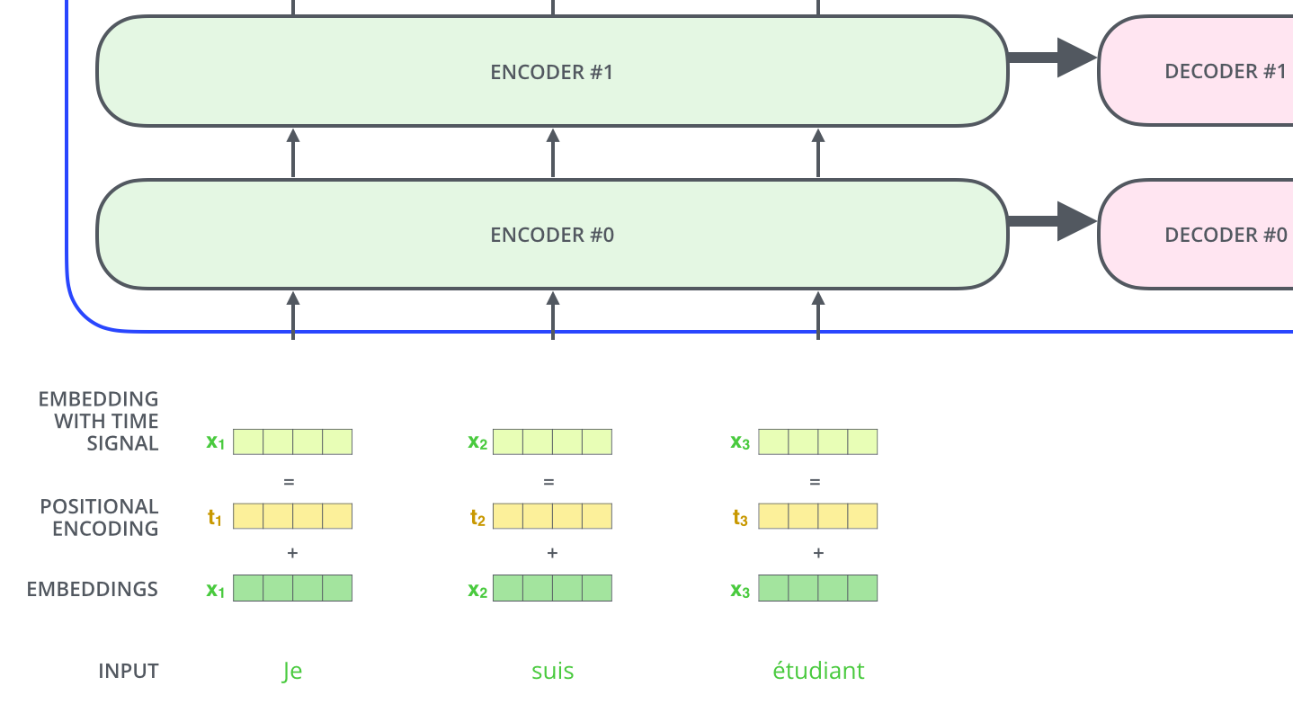 To give the model a sense of the order of the words, we add positional encoding vectors — the values of which follow a specific pattern.
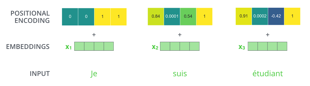
If we assumed the embedding has a dimensionality of 4, the actual positional encodings would look like this:
To give the model a sense of the order of the words, we add positional encoding vectors — the values of which follow a specific pattern.
If we assumed the embedding has a dimensionality of 4, the actual positional encodings would look like this:
 (View Highlight)
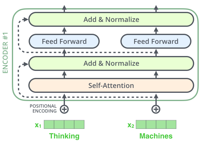
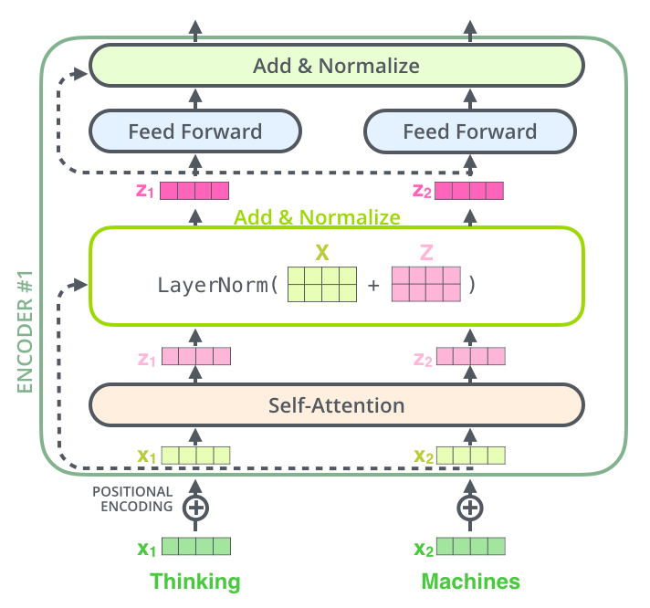
- One detail in the architecture of the encoder that we need to mention before moving on, is that each sub-layer (self-attention, ffnn) in each encoder has a residual connection around it, and is followed by a layer-normalization step.
 (View Highlight)
- If we’re to visualize the vectors and the layer-norm operation associated with self attention, it would look like this:
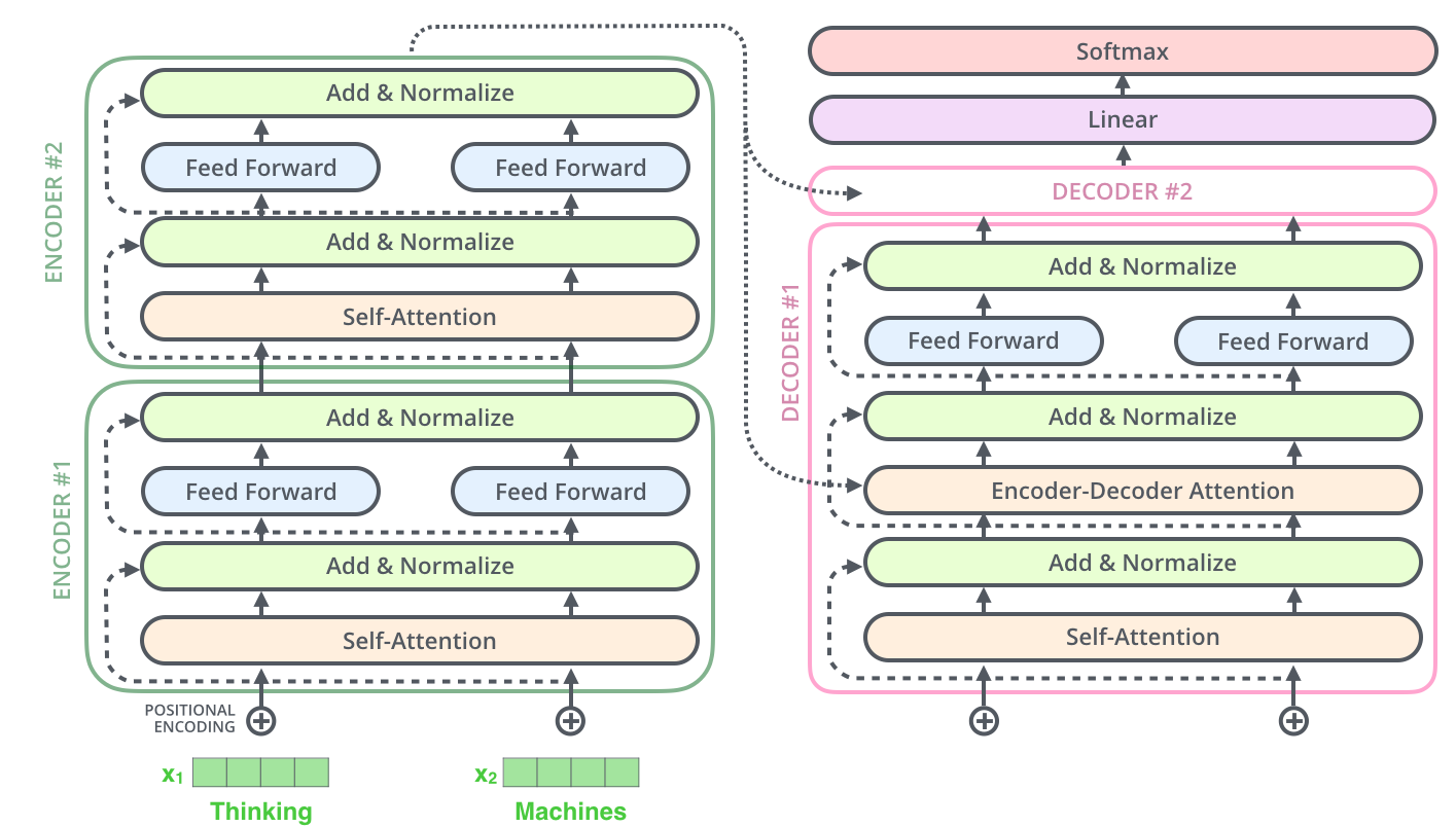
 This goes for the sub-layers of the decoder as well. If we’re to think of a Transformer of 2 stacked encoders and decoders, it would look something like this:
 (View Highlight)
- Now that we’ve covered most of the concepts on the encoder side, we basically know how the components of decoders work as well. But let’s take a look at how they work together.
The encoder start by processing the input sequence. The output of the top encoder is then transformed into a set of attention vectors K and V. These are to be used by each decoder in its “encoder-decoder attention” layer which helps the decoder focus on appropriate places in the input sequence: (View Highlight)
 (View Highlight)
- The following steps repeat the process until a special symbol is reached indicating the transformer decoder has completed its output. The output of each step is fed to the bottom decoder in the next time step, and the decoders bubble up their decoding results just like the encoders did. And just like we did with the encoder inputs, we embed and add positional encoding to those decoder inputs to indicate the position of each word.
 (View Highlight)
- The self attention layers in the decoder operate in a slightly different way than the one in the encoder:
In the decoder, the self-attention layer is only allowed to attend to earlier positions in the output sequence. This is done by masking future positions (setting them to
-inf) before the softmax step in the self-attention calculation.
The “Encoder-Decoder Attention” layer works just like multiheaded self-attention, except it creates its Queries matrix from the layer below it, and takes the Keys and Values matrix from the output of the encoder stack. (View Highlight)
- The decoder stack outputs a vector of floats. How do we turn that into a word? That’s the job of the final Linear layer which is followed by a Softmax Layer.
The Linear layer is a simple fully connected neural network that projects the vector produced by the stack of decoders, into a much, much larger vector called a logits vector.
Let’s assume that our model knows 10,000 unique English words (our model’s “output vocabulary”) that it’s learned from its training dataset. This would make the logits vector 10,000 cells wide – each cell corresponding to the score of a unique word. That is how we interpret the output of the model followed by the Linear layer.
The softmax layer then turns those scores into probabilities (all positive, all add up to 1.0). The cell with the highest probability is chosen, and the word associated with it is produced as the output for this time step. (View Highlight)
- Now that we’ve covered the entire forward-pass process through a trained Transformer, it would be useful to glance at the intuition of training the model.
During training, an untrained model would go through the exact same forward pass. But since we are training it on a labeled training dataset, we can compare its output with the actual correct output.
To visualize this, let’s assume our output vocabulary only contains six words(“a”, “am”, “i”, “thanks”, “student”, and “” (short for ‘end of sentence’)). (View Highlight)
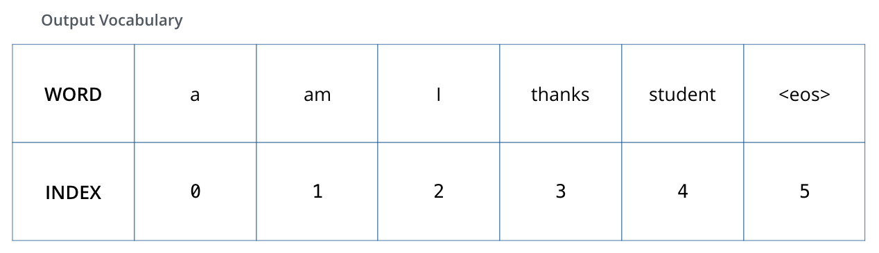 The output vocabulary of our model is created in the preprocessing phase before we even begin training. (View Highlight)
- Once we define our output vocabulary, we can use a vector of the same width to indicate each word in our vocabulary. This also known as one-hot encoding. So for example, we can indicate the word “am” using the following vector: (View Highlight)
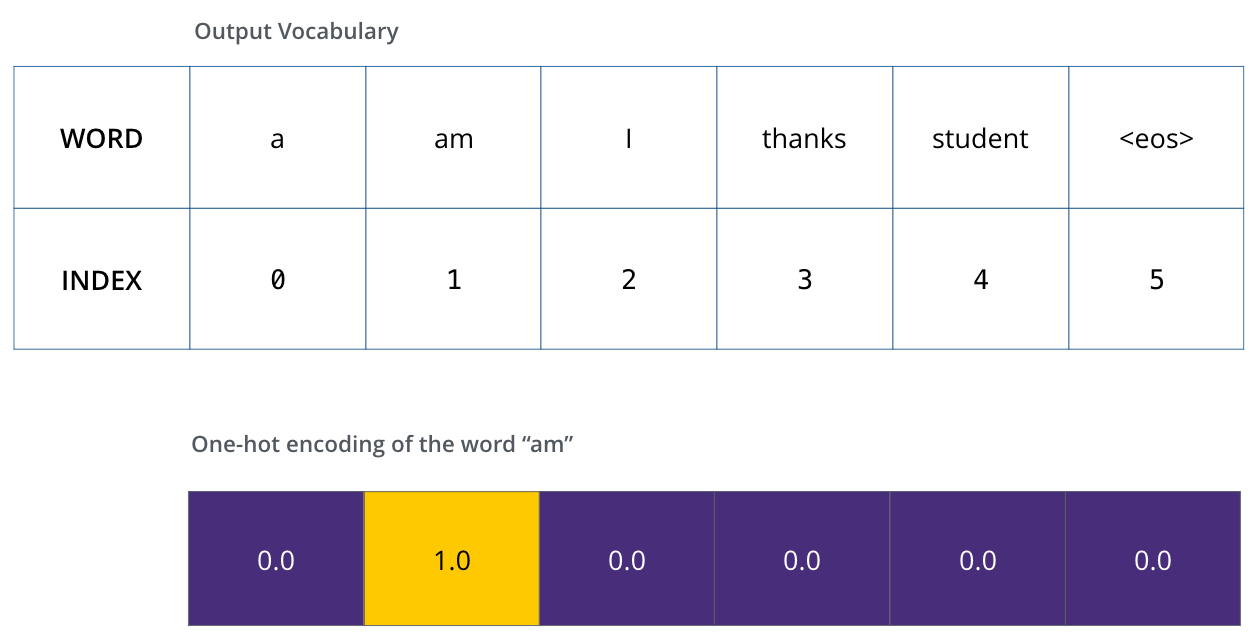 Example: one-hot encoding of our output vocabulary (View Highlight)
- The Loss Function
Say we are training our model. Say it’s our first step in the training phase, and we’re training it on a simple example – translating “merci” into “thanks”.
What this means, is that we want the output to be a probability distribution indicating the word “thanks”. But since this model is not yet trained, that’s unlikely to happen just yet.
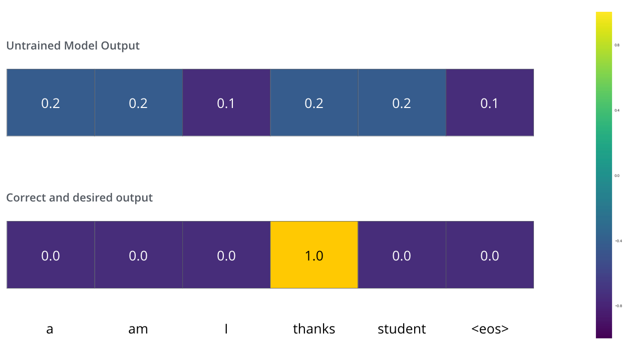 Since the model’s parameters (weights) are all initialized randomly, the (untrained) model produces a probability distribution with arbitrary values for each cell/word. We can compare it with the actual output, then tweak all the model’s weights using backpropagation to make the output closer to the desired output. (View Highlight)
- But note that this is an oversimplified example. More realistically, we’ll use a sentence longer than one word. For example – input: “je suis étudiant” and expected output: “i am a student”. What this really means, is that we want our model to successively output probability distributions where:
• Each probability distribution is represented by a vector of width vocab_size (6 in our toy example, but more realistically a number like 30,000 or 50,000)
• The first probability distribution has the highest probability at the cell associated with the word “i”
• The second probability distribution has the highest probability at the cell associated with the word “am”
• And so on, until the fifth output distribution indicates ‘
<end of sentence>’ symbol, which also has a cell associated with it from the 10,000 element vocabulary.
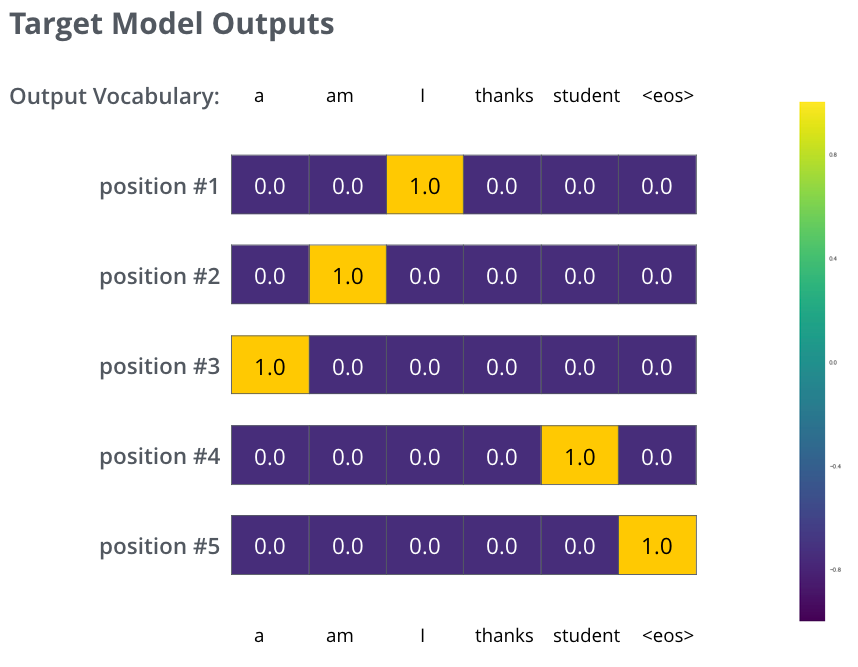 The targeted probability distributions we’ll train our model against in the training example for one sample sentence. (View Highlight)