
Metadata
- Author: Avi Chawla
- Full Title: The Motivation Behind Using KernelPCA Over PCA for Dimensionality Reduction
- URL: https://www.blog.dailydoseofds.com/p/the-motivation-behind-using-kernelpca
Highlights
- During dimensionality reduction, principal component analysis (PCA) tries to find a low-dimensional linear subspace that the given data conforms to. (View Highlight)
- It’s pretty clear from the above visual that there is a linear subspace along which the data could be represented while retaining maximum data variance. This is shown below: (View Highlight)
 (View Highlight)
- (View Highlight)
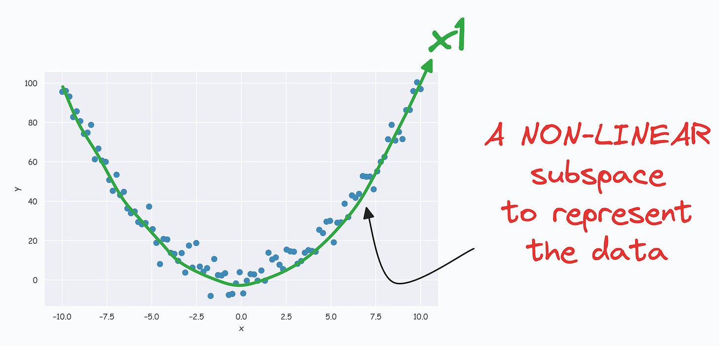
- The above curve is a continuous non-linear and low-dimensional subspace that we could represent our data given along. (View Highlight)
- The problem is that PCA cannot determine this subspace because the data points are non-aligned along a straight line. (View Highlight)
- Nonetheless, if we consider the above non-linear data, don’t you think there’s still some intuition telling us that this dataset can be reduced to one dimension if we can capture this non-linear curve. (View Highlight)
- Project the data to another high-dimensional space using a kernel function, where the data becomes linearly representable. Sklearn provides a KernelPCA wrapper, supporting many popularly used kernel functions. (View Highlight)
- Apply the standard PCA algorithm to the transformed data. (View Highlight)
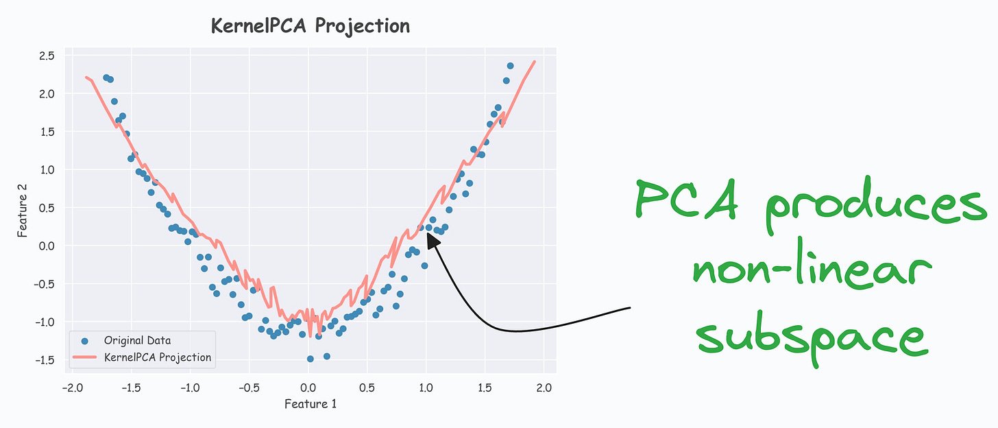
- As shown below, even though the data is non-linear, PCA still produces a linear subspace for projection:
 However, KernelPCA produces a non-linear subspace:
 (View Highlight)
 - The catch is the run time.
Please note that the run time of PCA is already cubically related to the number of dimensions.
 KernelPCA involves the kernel trick, which is quadratically related to the number of data points (
n). (View Highlight)