
Highlights §
- High-quality data is the fuel for modern data deep learning model training. Most of task-specific labeled data comes from human annotation, such as classification task or RLHF labeling (which can be constructed as classification format) for LLM alignment training. Lots of ML techniques in the post can help with data quality, but fundamentally human data collection involves attention to details and careful execution. The community knows the value of high quality data, but somehow we have this subtle impression that “Everyone wants to do the model work, not the data work” (Sambasivan et al. 2021).
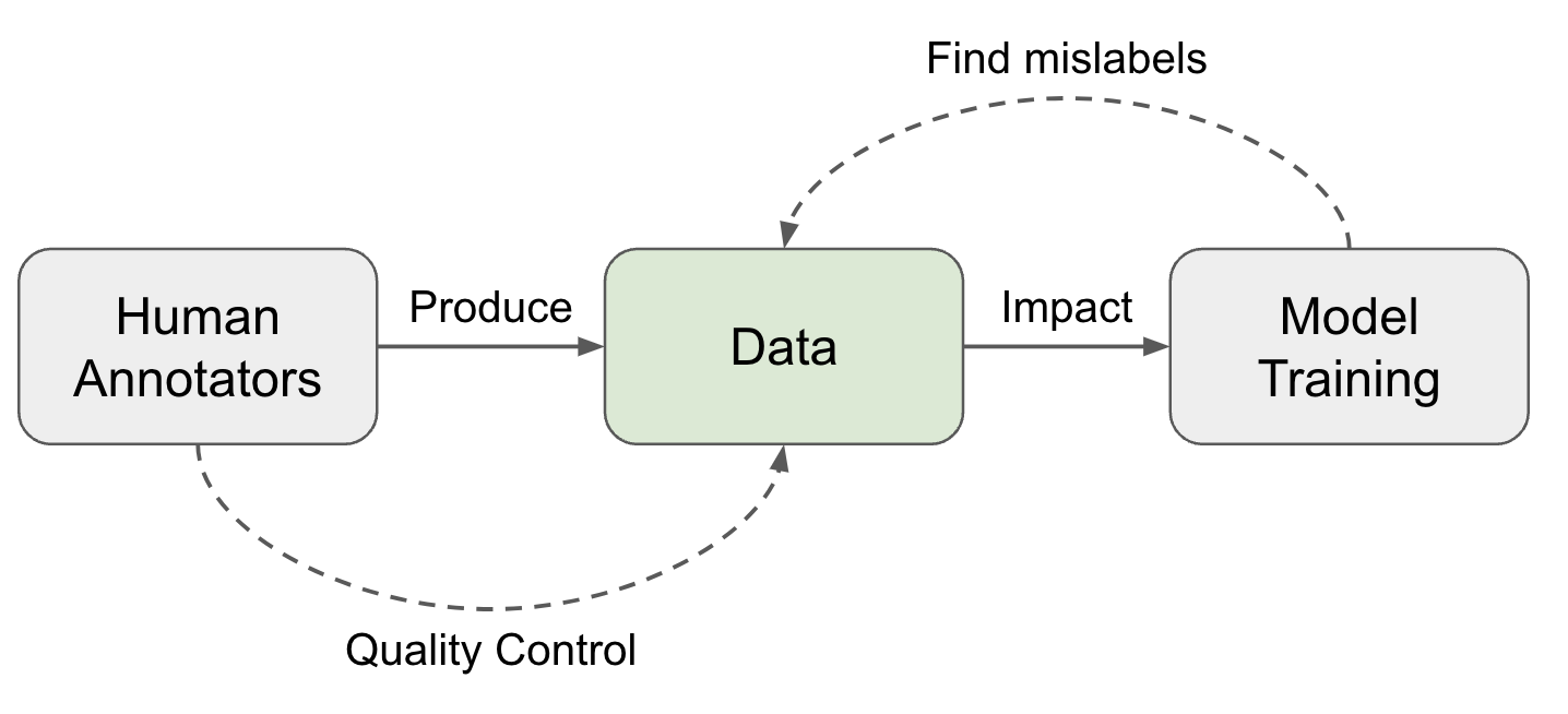 Fig. 1. Two directions to approach high data quality.
Human Raters ↔ Data Quality
Collecting human data involve a set of operation steps and every step contributes to the data quality:
Fig. 1. Two directions to approach high data quality.
Human Raters ↔ Data Quality
Collecting human data involve a set of operation steps and every step contributes to the data quality:
- Task Design: Design task workflow to improve clarity and reduce complexity. Detailed guidelines are helpful but very long and complicated guidelines demand a decent amount of training to be useful.
- Select and train a pool of raters: Select annotators with matched skillset and consistency. Training sessions are necessary. After onboarding, regular feedback and calibration sessions are also needed.
- Collect and aggregate data. This is the stage where more ML techniques can be applied to clean, filter and smartly aggregate data to identify the true labels.
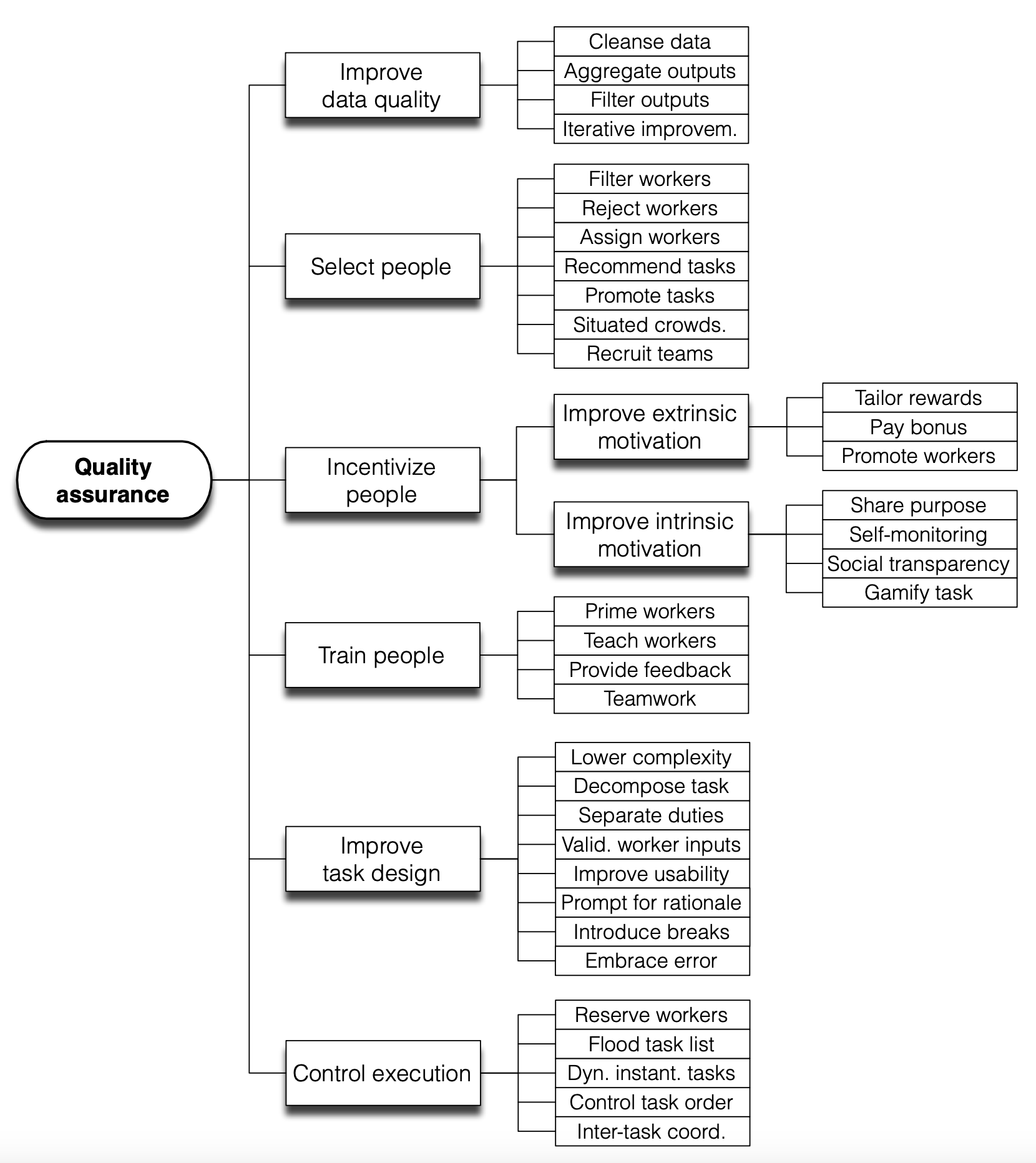 Fig. 2. Quality assurance refers to a set of actions that allow one to improve quality by acting on the quality attributes identified in the quality model. (Image source: Daniel et al. 2018)
The Wisdom of the Crowd
Vox populi(originally “Vox populi, vox Dei”), a Latin phrase, means the voice of people. A short paper named in it, published in 1907 on Nature tracked an event at an annual exhibition where a fat ox was selected and people would guess the weight of the ox in order to win a prize if the guess is close to the real number. The middlemost estimate was treated as “the vox populi” and ended up being very close to the true value. The author concluded “This result is, I think, more creditable to the trustworthiness of a democratic judgment than might have been expected.” This is probably the earliest mention of how crowdsourcing (“the wisdom of the crowd”) would work out.
Almost 100 years later, Callison-Burch (2009) did early work on using Amazon Mechanical Turk (AMT) to run non-expert human evaluation on Machine Translation (MT) tasks and even rely on non-experts to create new gold reference translation. The set up for human eval is simple: Each turker is shown a source sentence, a reference translation and 5 translations from 5 MT systems. They are asked to rank 5 translations from best to worst. Each task is completed by 5 turkers.
Unsurprisingly, there are spammers producing low quality annotation while only optimizing the volume. So when measuring the agreement between experts and non-experts, different weighting schemes can be applied to downweight the contribution of spammers: (1) “weighted by experts”: using agreement rate with experts on a gold set of 10 examples; (2) “weighted by non-experts”: relying on agreement rate with the rest of turkers on the whole dataset.
In a harder task, where non-expert human annotators are asked to create new gold reference translations. Callison-Burch designed two-stage tasks, where the first created new translations with reference to MT outputs and the second one to filter translations that look like from MT system. The correlation between expert and crowdsourced translations is higher than between expert and MT system outputs.
Fig. 2. Quality assurance refers to a set of actions that allow one to improve quality by acting on the quality attributes identified in the quality model. (Image source: Daniel et al. 2018)
The Wisdom of the Crowd
Vox populi(originally “Vox populi, vox Dei”), a Latin phrase, means the voice of people. A short paper named in it, published in 1907 on Nature tracked an event at an annual exhibition where a fat ox was selected and people would guess the weight of the ox in order to win a prize if the guess is close to the real number. The middlemost estimate was treated as “the vox populi” and ended up being very close to the true value. The author concluded “This result is, I think, more creditable to the trustworthiness of a democratic judgment than might have been expected.” This is probably the earliest mention of how crowdsourcing (“the wisdom of the crowd”) would work out.
Almost 100 years later, Callison-Burch (2009) did early work on using Amazon Mechanical Turk (AMT) to run non-expert human evaluation on Machine Translation (MT) tasks and even rely on non-experts to create new gold reference translation. The set up for human eval is simple: Each turker is shown a source sentence, a reference translation and 5 translations from 5 MT systems. They are asked to rank 5 translations from best to worst. Each task is completed by 5 turkers.
Unsurprisingly, there are spammers producing low quality annotation while only optimizing the volume. So when measuring the agreement between experts and non-experts, different weighting schemes can be applied to downweight the contribution of spammers: (1) “weighted by experts”: using agreement rate with experts on a gold set of 10 examples; (2) “weighted by non-experts”: relying on agreement rate with the rest of turkers on the whole dataset.
In a harder task, where non-expert human annotators are asked to create new gold reference translations. Callison-Burch designed two-stage tasks, where the first created new translations with reference to MT outputs and the second one to filter translations that look like from MT system. The correlation between expert and crowdsourced translations is higher than between expert and MT system outputs.
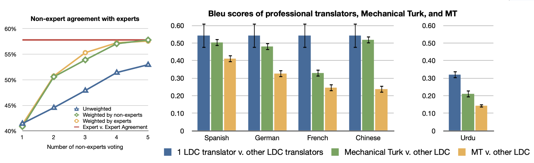 Fig. 3. (Left) Agreement is measured by comparing each pair of translation sentences (“A > B”, “A=B”, “A < B”) and thus chance agreement is 1/3. The upper bound is expert-expert agreement rate. (Right) LCD (Linguistic Data Consortium) translators provide expert translation. Comparison of BLEU score between translations of different sources. (Image source: Callison-Burch 2009)
Rater Agreement
In the prescriptive paradigm, we value one ground truth with consistent standards. The common practice is to collect multiple labels from multiple raters. Assuming each rater performs at a different level of quality, we can use a weighted average of annotations but weighted by a proficiency score, often approximated by how often they agree with others if no ground truth is available.
Majority Voting: Taking majority vote is the most simple way of aggregation, equivalent to taking the mode of a set of labels. In this setting, every annotator is treated equally.
Raw agreement (Tratz & Hovy, 2010): Per annotation, raw agreement counts the percentage of other people agreeing with them. This is indirectly correlated to majority vote, because all members of the majority class are expected to get higher inter-annotator agreement rate.
Cohen’s Kappa (Landis & Koch, 1977): Cohen’s kappa measures the inter-rater agreement in the form of κ=(p0−pe)/(1−pc), where po is the raw agreement rate and pe is the agreement by chance. Cohen’s kappa has a correction term for agreeing by chance, but this correction may be overestimated if one label is more prevalent.
Probabilistic Graph Modeling: There is a body of work relying on probabilistic graph modeling to model different factors within annotation decisions, e.g. difficulty of the task, task latent topics, rater bias, rater confidence, and then predict the true labels accordingly. Zheng et al. (2017) compared 17 algorithms on truth inference in crowdsourcing and most of them are probabilistic graph models.
• MACE( Multi-Annotator Competence Estimation; Hovy et al. 2013) is an early example of using graph modeling to estimate the likelihood of someone acting like a “spammer” by providing random labels. Unsurprisingly in cases when the incentive is misaligned, some annotators may behave as “spammers” to optimize the volume of tasks completed for higher pay. The goal of MACE is to identify spammers. Given a task i and an annotator j, Ti is the true label, Aij is the assigned label and Sij models the probability of annotator j is spamming. Then the generative process can be represented as belows. The parameter θj defines the trustworthiness of the annotator j (probability of not spamming) and the parameter ξj defines how an annotator behaves when they are spamming.
for i=1…N:Ti∼Uniformfor j=1…M:Sij∼Bernoulli(1−θj)if Sij=0:Aij=Tielse :Aij∼Multinomial(ξj)
Then we can learn θ,ξ to maximize the observed data, in the form of the marginal data likelihood, where A is the matrix of annotations, S is the matrix of competence indicators and T is the matrix of true labels:
P(A;θ,ξ)=∑T,S[∏i=1NP(Ti)⋅∏j=1MP(Sij;θj)⋅P(Aij|Sij,Ti;ξj)]
Either EM (Expectation–maximization) or VB (Variational Bayes) can be applied to maximize the above marginal likelihood. During EM optimization, at M-step, a fixed value δ is added to the fractional counts before normalizing. During VB training, they applied symmetric Beta priors on θj and symmetric Dirichlet priors on ξj. When recovering the correct answers, we can take majority vote weighted by the annotators’ θ estimates.
Rater Disagreement & Two Paradigms
The aggregation based rater agreement described above depends on an assumption that there exists a gold answer to compare with and thus we can evaluate annotators’ performance accordingly. However in many topics, especially in safety, social, or cultural areas, (View Highlight)
Fig. 3. (Left) Agreement is measured by comparing each pair of translation sentences (“A > B”, “A=B”, “A < B”) and thus chance agreement is 1/3. The upper bound is expert-expert agreement rate. (Right) LCD (Linguistic Data Consortium) translators provide expert translation. Comparison of BLEU score between translations of different sources. (Image source: Callison-Burch 2009)
Rater Agreement
In the prescriptive paradigm, we value one ground truth with consistent standards. The common practice is to collect multiple labels from multiple raters. Assuming each rater performs at a different level of quality, we can use a weighted average of annotations but weighted by a proficiency score, often approximated by how often they agree with others if no ground truth is available.
Majority Voting: Taking majority vote is the most simple way of aggregation, equivalent to taking the mode of a set of labels. In this setting, every annotator is treated equally.
Raw agreement (Tratz & Hovy, 2010): Per annotation, raw agreement counts the percentage of other people agreeing with them. This is indirectly correlated to majority vote, because all members of the majority class are expected to get higher inter-annotator agreement rate.
Cohen’s Kappa (Landis & Koch, 1977): Cohen’s kappa measures the inter-rater agreement in the form of κ=(p0−pe)/(1−pc), where po is the raw agreement rate and pe is the agreement by chance. Cohen’s kappa has a correction term for agreeing by chance, but this correction may be overestimated if one label is more prevalent.
Probabilistic Graph Modeling: There is a body of work relying on probabilistic graph modeling to model different factors within annotation decisions, e.g. difficulty of the task, task latent topics, rater bias, rater confidence, and then predict the true labels accordingly. Zheng et al. (2017) compared 17 algorithms on truth inference in crowdsourcing and most of them are probabilistic graph models.
• MACE( Multi-Annotator Competence Estimation; Hovy et al. 2013) is an early example of using graph modeling to estimate the likelihood of someone acting like a “spammer” by providing random labels. Unsurprisingly in cases when the incentive is misaligned, some annotators may behave as “spammers” to optimize the volume of tasks completed for higher pay. The goal of MACE is to identify spammers. Given a task i and an annotator j, Ti is the true label, Aij is the assigned label and Sij models the probability of annotator j is spamming. Then the generative process can be represented as belows. The parameter θj defines the trustworthiness of the annotator j (probability of not spamming) and the parameter ξj defines how an annotator behaves when they are spamming.
for i=1…N:Ti∼Uniformfor j=1…M:Sij∼Bernoulli(1−θj)if Sij=0:Aij=Tielse :Aij∼Multinomial(ξj)
Then we can learn θ,ξ to maximize the observed data, in the form of the marginal data likelihood, where A is the matrix of annotations, S is the matrix of competence indicators and T is the matrix of true labels:
P(A;θ,ξ)=∑T,S[∏i=1NP(Ti)⋅∏j=1MP(Sij;θj)⋅P(Aij|Sij,Ti;ξj)]
Either EM (Expectation–maximization) or VB (Variational Bayes) can be applied to maximize the above marginal likelihood. During EM optimization, at M-step, a fixed value δ is added to the fractional counts before normalizing. During VB training, they applied symmetric Beta priors on θj and symmetric Dirichlet priors on ξj. When recovering the correct answers, we can take majority vote weighted by the annotators’ θ estimates.
Rater Disagreement & Two Paradigms
The aggregation based rater agreement described above depends on an assumption that there exists a gold answer to compare with and thus we can evaluate annotators’ performance accordingly. However in many topics, especially in safety, social, or cultural areas, (View Highlight)
- To capture systematic disagreement among annotators when learning to predict labels, Davani et al. (2021) experimented with a multi-annotator model where predicting each annotator’s labels is treated as one sub-task. Say, the classification task is defined on an annotated dataset D=(X,A,Y), where X is the text instances, A is the set of annotators and Y is the annotation matrix, yij∈Y represents a binary label assigned by aj∈A to the sample xi∈X. The majority vote for xi is denoted as y¯i,. (View Highlight)
- Jury Learning (Gordon et al. 2022) mimics the jury process by modeling the different annotators’ labeling behavior conditioned on their characteristics. Starting with a dataset with labels and demographic characteristics of each labeler, we train a model to learn to predict labels made by every individual annotator, each as a potential juror. At decision time, practitioners can specify the composition of a group of jurors to determine a sampling strategy. The final decision is made by aggregating labels from jurors from multiple trials.
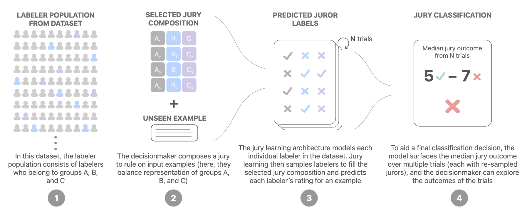 Fig. 7. Illustration of how jury learning works. (Image source: (View Highlight)
- Once a dataset is constructed, there are methods to help us identify mistakenly labeled samples according to model training dynamics. Note that we only focus on methods to find and exclude data points with potentially incorrect labels, not about how to train a model with noisy data. (View Highlight)
- Influence functions is a classic technique from robust statistics (Hampel, 1974) to measure the effect of training data points by describing how the model parameters change as we upweight a training point by an infinitesimal amount. Koh & Liang (2017) proposed a way to approximate the influence functions in deep neural networks. (View Highlight)
- Using the influence function we can measure the effect of a single data point on model parameters and loss function in closed forms. It can help approximate leave-one-out retraining without actually running all the retraining. To identify mislabeled data, we can measure Iup,loss(zi,zi), approximating the prediction error on zi if zi is removed from the training set.
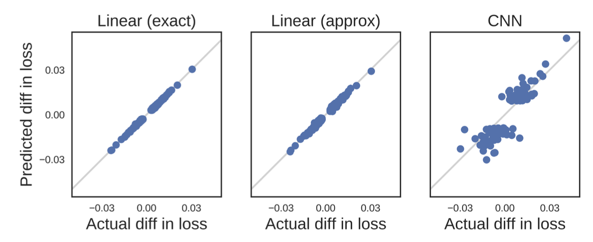 Fig. 10. Influence functions values match leave-one-out training results on 10-class MNIST. (Image source: Kohn & Liang, 2017)
Given the closed form, influence functions is still hard to be scaled up because the inverse Hessian vector product is hard to compute. Grosse et al. (2023) experimented with the EK-FAC (Eigenvalue-corrected Kronecker-Factored Approximate Curvature; George et al. 2018) approximation instead. (View Highlight)
Fig. 10. Influence functions values match leave-one-out training results on 10-class MNIST. (Image source: Kohn & Liang, 2017)
Given the closed form, influence functions is still hard to be scaled up because the inverse Hessian vector product is hard to compute. Grosse et al. (2023) experimented with the EK-FAC (Eigenvalue-corrected Kronecker-Factored Approximate Curvature; George et al. 2018) approximation instead. (View Highlight)
- Another branch of methods are to track the changes of model prediction during training to identify cases which seem hard to be learned. Data Maps (Swayamdipta et al. 2020) tracks two attributes of model behavior dynamics during training to analyze the quality of dataset:
- Confidence: The model’s confidence in the true label, defined as the mean model probability of the true label across epochs. They also used a coarse-grained metric, “correctness”, defined as the fraction of times when the model predicts the correct label across epochs.
- Variability: The variation of the confidence, defined as the standard deviation of model probability of the true label across epochs.
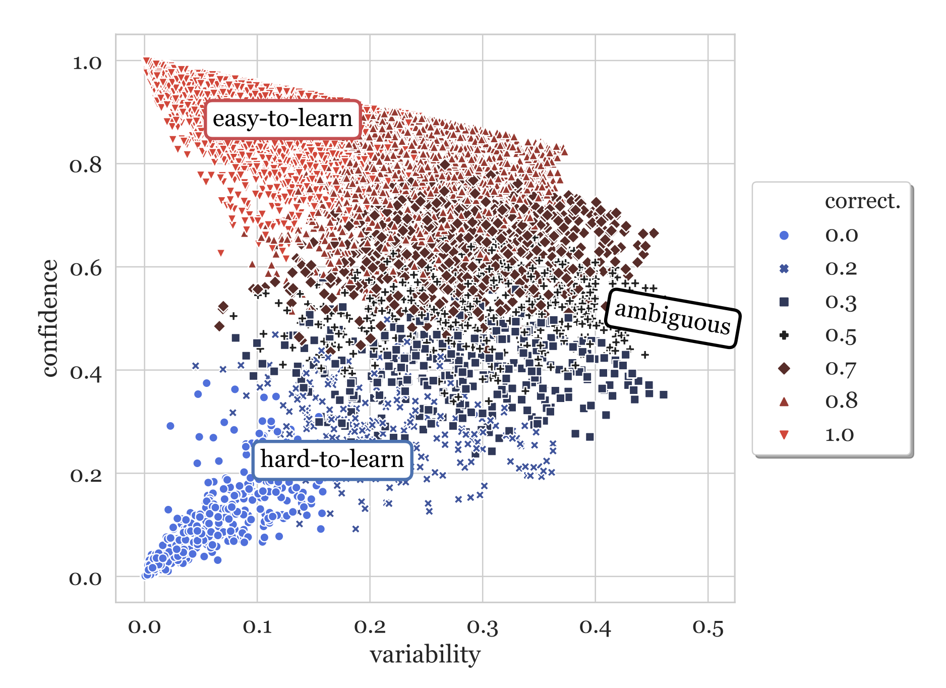 Fig. 11. Data map for SNLI training set, based on a RoBERTa classifier. (Image source: Swayamdipta et al. 2020) (View Highlight)
- Hard-to-learn (low confidence, low variability) samples are more likely to be mislabeled. They ran an experiment on WinoGrande dataset with 1% flipped label data. After retraining, flipped instances move to the lower confidence and slightly higher variability regions, indicating that the hard-to-learn regions contains mislabeled samples. Given this, we can train a classifier on equal numbers of label flipped and clean samples using only the confidence score (unsure why the paper didn’t use both confidence and variability as features). This simple noise classifier then can be used on the original dataset to identify potentially mislabeled instances.
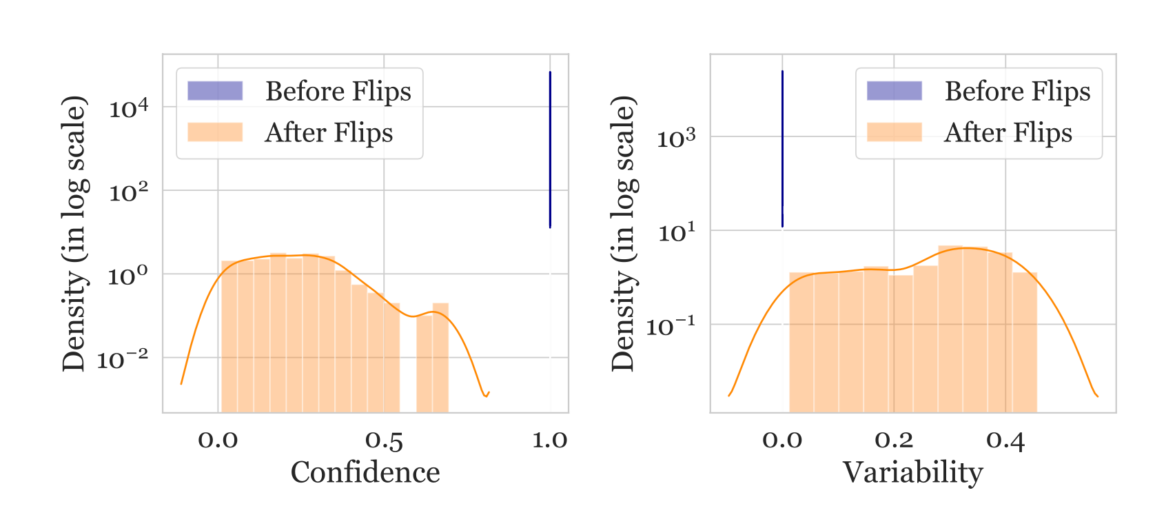 Fig. 12. Data points originally with high confidence and low variability scores moved to low confidence, slightly higher variability regions after labels get flipped. (Image source: Swayamdipta et al. 2020)
However, we should not consider all hard-to-learn samples to be incorrect. In fact, the paper hypothesizes that ambiguous (high variability) and hard-to-learn (low confidence, low variability) samples are more informative for learning. Experiments showed that they are good for OOD generalization, giving better results on OOD eval, even in comparison to 100% training set. (View Highlight)
Fig. 12. Data points originally with high confidence and low variability scores moved to low confidence, slightly higher variability regions after labels get flipped. (Image source: Swayamdipta et al. 2020)
However, we should not consider all hard-to-learn samples to be incorrect. In fact, the paper hypothesizes that ambiguous (high variability) and hard-to-learn (low confidence, low variability) samples are more informative for learning. Experiments showed that they are good for OOD generalization, giving better results on OOD eval, even in comparison to 100% training set. (View Highlight)
- To investigate whether neural networks have a tendency to forget previously learned information, Mariya Toneva et al. (2019) designed an experiment: They track the model prediction for each sample during the training process and count the transitions for each sample from being classified correctly to incorrectly or vice-versa. Then samples can be categorized accordingly,
• Forgettable (redundant) samples: If the class label changes across training epochs.
• Unforgettable samples: If the class label assignment is consistent across training epochs. Those samples are never forgotten once learned.
They found that there are a large number of unforgettable examples that are never forgotten once learnt. Examples with noisy labels or images with “uncommon” features (visually complicated to classify) are among the most forgotten examples. The experiments empirically validated that unforgettable examples can be safely removed without compromising model performance.
In the implementation, the forgetting event is only counted when a sample is included in the current training batch; that is, they compute forgetting across presentations of the same example in subsequent mini-batches. The number of forgetting events per sample is quite stable across different seeds and forgettable examples have a small tendency to be first-time learned later in the training. The forgetting events are also found to be transferable throughout the training period and between architectures. (View Highlight)
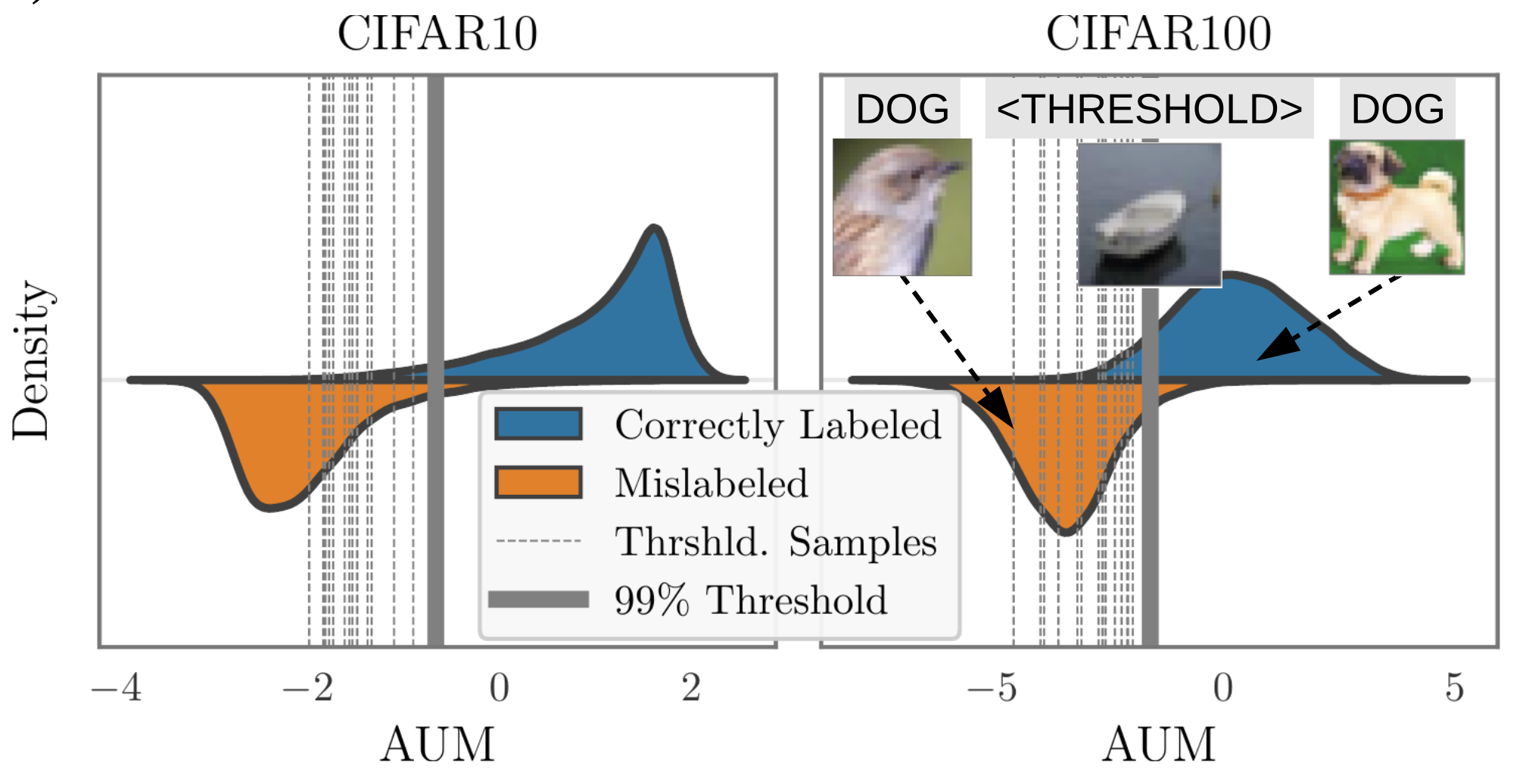
- Pleiss, et al. (2020) developed a method named AUM (Area under the Margin) to spot wrong labels based on such an assumption: Say, a BIRD image is mistakenly marked as DOG. The gradient update would encourage generalization from other BIRD images to this BIRD image, while the DOG label provides an incorrect supervised signal to encourage the update to go another way. Hence, there exists tension between generalization and (wrong) prediction in gradient update signals. (View Highlight)
- In order to determine the threshold, they insert fake data, named “threshold samples”, to determine the threshold:
- Create a subset of threshold samples Dthr. If there are N training samples for C classes, we randomly sample N/(C+1) samples and switch all their labels to a fake new class C+1.
- Merge threshold samples into the original dataset: D′=(x,C+1):x∈Dthr∪(D∖Dthr);
- Train the model on D′ and measure AUM of all the data;
- Compute the threshold α as the 99th percentile of AUM of threshold samples;
- Identify mislabeled data using α a threshold: (x,y)∈D∖Dthr:AUMx,y≤α
 (View Highlight)
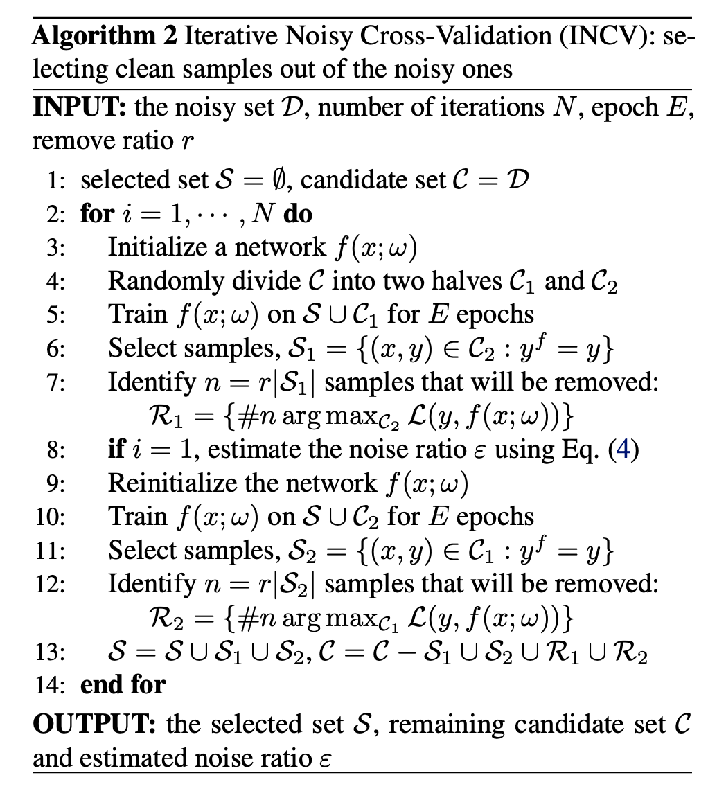
- The NCV (Noisy Cross-Validation) method (Chen et al. 2019) divides the dataset into half at random, and then identifies data samples as “clean” if its label matches the predicted label provided by the model that is only trained on the other half of the dataset. Clean samples are expected to be more trustworthy. INCV (Iterative Noisy Cross-Validation) runs NCV iteratively where more clean samples are added into the trusted candidate set C and more noisy samples are removed.
 (View Highlight)